Planet Haskell

October 21, 2025

Abhinav Sarkar

A Fast Bytecode VM for Arithmetic: The Virtual Machine

In this series of posts, we write a fast bytecode compiler and a virtual machine for arithmetic in Haskell. We explore the following topics:

In this final post, we write the virtual machine that executes our bytecode, and benchmark it.

This post was originally published on abhinavsarkar.net.

This post is part of the series: A Fast Bytecode VM for Arithmetic.

  1. The Parser
  2. The Compiler
  3. The Virtual Machine (you are here)

Introduction

Bytecode Virtual Machines (VMs) are known to be faster than AST-walking interpreters. That’s why many real-world programming languages these days are implemented with bytecode VMs, for example, Java, Python, PHP, and Raku. The reason is partially, the flat and compact nature of bytecode itself. But VMs also have a few other tricks up their sleeves that make them highly performant. In this post, we write a VM for our arithmetic expression language, and explore some of these performance tricks.

But first, we need to finish a pending task.

Testing the Compiler

We wrote some unit tests for our compiler in the last post, but unit tests cover only the cases we can think of. A compiler has to deal with any input, and with just unit tests we cannot be sure of its correctness.

To test our compiler and other components for correctness, we use the QuickCheck library. QuickCheck is a Property-based Testing framework. The key idea of property-based testing is to write properties of our code that hold true for any input, and then to automatically generate a large number of arbitrary inputs and make sure that the properties are indeed true for them12. Since we are writing an arithmetic expression parser/compiler/VM, we generate arbitrary expression ASTs, and use them to assert certain invariants of our program.

With QuickCheck, we write generators for the inputs for our tests. These generators are composable just like parser combinators are. We use the library provided generators to write small generators that we combine to create larger ones. Let’s start:

numGen :: Q.Gen Expr
numGen = Num <$> Q.arbitrary

varGen :: Set.Set Ident -> Q.Gen Expr
varGen vars = Var <$> Q.elements (Set.toList vars)
 
identGen :: Q.Gen Ident
identGen =
  mkIdent
    <$> ( (:)
            <$> Q.elements lower
            <*> Q.resize 5 (Q.listOf1 $ Q.elements validChars)
        ) `Q.suchThat` (not . isReservedKeyword . BSC.pack)
  where
    lower = ['a' .. 'z']
    validChars = lower <> ['A' .. 'Z']
ArithVMLib.hs

First come the basic generators:

  • numGen generates number expressions by using QuickCheck’s built-in arbitrary function.
  • varGen generates variable expressions by choosing from the set of passed valid variable names.
  • identGen generates valid identifiers from combinations of letters a—z and A—Z, and discarding ones that are reserved keywords.

Moving on to composite generators:

binOpGen :: Set.Set Ident -> Int -> Q.Gen Expr
binOpGen vars size =
  BinOp
    <$> Q.chooseEnum (Add, Div)
    <*> exprGen vars (size `div` 2)
    <*> exprGen vars (size `div` 2)

letGen :: Set.Set Ident -> Int -> Q.Gen Expr
letGen vars size = do
  x <- identGen
  let vars' = Set.insert x vars
  Let x <$> exprGen vars (size `div` 2) <*> exprGen vars' (size `div` 2)

exprGen :: Set.Set Ident -> Int -> Q.Gen Expr
exprGen vars size
  | size < 5 = Q.frequency [(4, Q.oneof baseGens), (1, Q.oneof compositeGens)]
  | otherwise = Q.frequency [(1, Q.oneof baseGens), (4, Q.oneof compositeGens)]
  where
    baseGens = numGen : [varGen vars | not $ Set.null vars]
    compositeGens = [binOpGen vars size, letGen vars size]
ArithVMLib.hs
  • binOpGen generates binary expressions with arbitrary binary operations. It recursively calls exprGen to generate the operands. The size parameter controls the complexity of the generated expressions, and we half the size of operands (and so on recursively) so that we don’t end up with infinitely large expressions.

  • letGen generates Let expressions by generating an identifier, and then generating the assignment and body expressions recursively. We do the same trick of halving sizes here as well. Notice that the assignment is generated with the passed variable names in scope, whereas the body is generated with the new identifier added to the scope.

  • exprGen uses the above generators to generate all kinds of expressions. At smaller sizes, it prefers to generate base expressions, while at larger sizes, it prefers composite ones. Due to the careful recursive halving of size in composite generators, we end up with expressions of finite sizes.

Finally, we have some instances of QuickCheck’s Arbitrary type class to tie everything together:

instance Q.Arbitrary Expr where
  arbitrary = Q.sized $ exprGen Set.empty
  shrink = Q.genericShrink

instance Q.Arbitrary Ident where
  arbitrary = identGen

instance Q.Arbitrary Op where
  arbitrary = Q.chooseEnum (Add, Div)
ArithVMLib.hs

We can apply them in GHCi:

> :set -XTypeApplications
> Q.sample $ Q.arbitrary @Expr
0
((let jgSg = 2 in (-2 - -2)) + -2)
2
(0 / 1)
(-11 / -13)
((let kpuS = 10 in 31) + (let jChmZV = -12 in jChmZV))
((54 * -55) * (let ohLSk = 29 in -45))
(-102 - (-119 * -125))
(-234 - (32 / -217))
(let kVrB = (-261 * 238) in ((let qdz = 228 in 347) + 18))
(let uMMdXH = ((let ePUi = 842 in ePUi) - (let zrkM = (let vwH = ((9 + -987) / -487) in (let ylKowr = vwH in vwH)) in zrkM)) in (((uMMdXH / -836) / uMMdXH) - (let qkK = uMMdXH in qkK)))

Notice that the generated samples increase in complexity. With the generators in place, we define our properties next. Let’s test our parser first:

prop_print_ast_then_parse_returns_same_ast :: Spec
prop_print_ast_then_parse_returns_same_ast =
  prop "Property: Print AST then parse returns same AST" $ \expr ->
    parse (BSC.pack $ show expr) == Right expr
ArithVMSpec.hs

This property is a simple round-trip test for the parser and printer: we parse the string representation of a generated expression, and assert that it gives back the same expression.

The second property is a more involved round-trip test for the compiler and decompiler:

prop_disassemble_bytecode_then_decompile_then_compile_returns_same_bytecode :: Spec
prop_disassemble_bytecode_then_decompile_then_compile_returns_same_bytecode =
  prop ( "Property: Disassemble bytecode then decompile then compile"
         <> " returns same bytecode" ) $ \expr ->
    case compile (sizedExpr expr) of
      Left _ -> Q.discard
      Right bytecode ->
        (disassemble bytecode >>= (decompile >>> fmap sizedExpr) >>= compile)
          == Right bytecode
ArithVMSpec.hs

This asserts that compiling an expression, then disassembling and decompiling it, and finally compiling it again should result in the original bytecode3.

This requires a helper function to get the size of an expression:

sizedExpr :: Expr -> SizedExpr
sizedExpr expr = case expr of
  Num _ -> (expr, 3)
  Var _ -> (expr, 2)
  BinOp _ a b -> (expr, snd (sizedExpr a) + snd (sizedExpr b) + 1)
  Let _ a b -> (expr, snd (sizedExpr a) + snd (sizedExpr b) + 1)
ArithVMLib.hs

We run these tests in a later section. This ends our short detour.

The Virtual Machine

Now for the main event: the virtual machine. Our VM is a stack-based machine that operates on a stack of values and executes the compiled bytecode. Our goal is to be as fast as possible. For a quick reminder, these are our Opcodes:

data Opcode
  = OPush !Int16        -- 0
  | OGet !Word8         -- 1
  | OSwapPop            -- 2
  | OAdd                -- 3
  | OSub                -- 4
  | OMul                -- 5
  | ODiv                -- 6
  deriving (Show, Read, Eq, Generic)
ArithVMLib.hs

And now, the heart of the VM:

interpretBytecode :: Bytecode -> Result Int16
interpretBytecode = interpretBytecode' defaultStackSize

interpretBytecode' :: Int -> Bytecode -> Result Int16
interpretBytecode' stackSize bytecode = runST $ runExceptT $ do
  stack <- PA.newPinnedPrimArray stackSize
  sp <- go 0 0 stack
  checkStack InterpretBytecode stackSize sp
  PA.readPrimArray stack 0
  where
    !size = BS.length bytecode

    go sp ip _ | ip == size = pure sp
    go !sp !ip stack = do
      let opcode = readInstr bytecode ip
      if
        | sp >= stackSize -> throwInterpretError "Stack overflow"
        | sp < 0 -> throwInterpretError "Stack underflow"
        | sp < 2 && opcode >= 2 -> throwInsufficientElementsError
        | opcode == 0 && ip + 2 >= size -> throwIPOOBError $ ip + 2
        | opcode == 1 && ip + 1 >= size -> throwIPOOBError $ ip + 1
        | otherwise -> case opcode of
            0 -> do                 -- OPush
              PA.writePrimArray stack sp $ readInstrArgInt16 bytecode ip
              go (sp + 1) (ip + 3) stack
            1 -> do                 -- OGet
              let i = fromIntegral $ readInstrArgWord8 bytecode ip
              if i < sp
                then do
                  PA.copyMutablePrimArray stack sp stack i 1
                  go (sp + 1) (ip + 2) stack
                else throwInterpretError $
                  "Stack index " <> show i <> " out of bound " <> show (sp - 1)
            2 -> do                 -- OSwapPop
              PA.copyMutablePrimArray stack (sp - 2) stack (sp - 1) 1
              go (sp - 1) (ip + 1) stack
            3 -> interpretBinOp (+) -- OAdd
            4 -> interpretBinOp (-) -- OSub
            5 -> interpretBinOp (*) -- OMul
            6 -> do                 -- ODiv
              b <- PA.readPrimArray stack $ sp - 1
              a <- PA.readPrimArray stack $ sp - 2
              when (b == 0) $ throwInterpretError "Division by zero"
              when (b == (-1) && a == minBound) $
                throwInterpretError "Arithmetic overflow"
              PA.writePrimArray stack (sp - 2) $ a `div` b
              go (sp - 1) (ip + 1) stack
            n -> throwInterpretError $
              "Invalid bytecode: " <> show n <> " at: " <> show ip
      where
        interpretBinOp op = do
          b <- PA.readPrimArray stack $ sp - 1
          a <- PA.readPrimArray stack $ sp - 2
          PA.writePrimArray stack (sp - 2) $ a `op` b
          go (sp - 1) (ip + 1) stack
        {-# INLINE interpretBinOp #-}

        throwIPOOBError ip = throwInterpretError $
          "Instruction index " <> show ip <> " out of bound " <> show (size - 1)

        throwInsufficientElementsError =
          throwInterpretError "Not enough elements to execute operation"

        throwInterpretError = throwError . Error InterpretBytecode
ArithVMLib.hs

The interpretBytecode' function is where the action happens. It is way more complex than interpretAST, but the complexity has a reason, namely performance.

interpretBytecode' runs inside the ST monad wrapped with the ExceptT monad transformer. ST monad lets us use mutable data structures locally while ensuring the function remains externally pure. ExceptT monad transformer adds support for throwing and propagating errors in a pure manner.

We use PrimArray for our stack, which is a mutable array of unboxed primitive types, in our case an array of Int16 values. Using a mutable unboxed array is much faster than using an immutable and/or boxed one like Seq or Vector due to reduced allocation and/or pointer chasing.

The core of the VM is the go function, a tight, tail-recursive loop that GHC compiles into an efficient machine loop, as we see later. It takes the stack pointer (sp), instruction pointer (ip)4, and the stack as arguments.

At the top of each loop, a block of guard clauses checks for stack overflow, underflow, and other error conditions before branching on the current opcode. Placing these checks at the top instead of inside the opcode cases is a deliberate choice. This may make the code slightly harder to understand, but it significantly improves the performance of the loop by moving all branching at the beginning of the loop, resulting in code that is more friendly to the CPU’s Branch Predictor. Also notice how we reduce the number of checks by working with a range of opcodes at once in the opcode >= 2 guard. The checks are also sorted so as to be most performant, guided by profiling and benchmarking5.

The handling of each opcode is actually pretty straightforward. We use different PrimArray specific operations to read and write to the stack, while taking care of doing the required bound and arithmetic checks. We also use the readInstr* functions that we wrote earlier.

After carrying out each operation, we reenter the loop by calling it tail-recursively with the right stack and instruction pointers. Finally, we make sure that the execution terminated correctly by checking the state of the stack, and return its first element.

Peeking Under the Hood: GHC Core

We see later that the VM is quite fast, but how does GHC achieve this performance? To see the magic, we can look at GHC’s intermediate language: Core. Core is a simpler functional language than Haskell to which GHC compiles Haskell. The simpler nature of Core makes it easier for GHC to optimize it, and compile it further. We can get the Core code for a program by compiling with the GHC option -ddump-simpl.

The actual Core code for our VM is too verbose to show here, but here is a simplified C-like pseudo-code version of our go loop:

$wgo (stack_addr, ip, sp) {
  if (ip == bytecode_size) {
    return sp;
  }
  if (sp >= stack_size) {
    throw "Stack Overflow";
  }
  if (sp < 0) {
    throw "Stack Underflow";
  }

  opcode = read_byte_at(bytecode_addr, ip);
  // ... other checks ...

  switch (opcode) {
    case 0: // OPush
      val = read_int16_at(bytecode_addr, ip + 1);
      write_int16_at(stack_addr, sp, val);
      jump $wgo(stack_addr, ip + 3, sp + 1);

    case 3: // OAdd
      val2 = read_int16_at(stack_addr, sp - 1);
      val1 = read_int16_at(stack_addr, sp - 2);
      write_int16_at(stack_addr, sp - 2, val1 + val2);
      jump $wgo(stack_addr, ip + 1, sp - 1);

    // ... other cases ...
  }
}

A few key optimizations are worth pointing out:

  1. The loop: The tail-recursive go function is compiled into a proper loop. The jump $wgo(...) instruction is effectively a goto, which means there’s no function call overhead for each iteration of the VM loop.

  2. Unboxing: The Core code is full of primitive, unboxed types like Int#, Addr#, and Word#, and operations on them. These are raw machine integers and memory addresses, not boxed Haskell objects. This means operations on them are as fast as they would be in C. The stack operations are not function calls on a PrimArray instance, but primitive memory reads and writes on a raw memory address stack_addr.

  3. Inlining: The interpretBinOp helper function is completely inlined into the main loop. For OAdd, the code for reading two values, adding them, and writing the result is laid out inline, and works on unboxed values and array address.

In short, GHC has turned our high-level, declarative Haskell code into a low-level loop that looks remarkably like one we would write in C. We get the safety and expressiveness of Haskell, while GHC does the heavy lifting to produce highly optimized code. It’s the best of both worlds!

Testing the VM

We must test the VM to make sure it works correctly6. We reuse the success and failure tests for the AST interpreter, as the bytecode interpreter should yield the same result:

bytecodeInterpreterSpec :: Spec
bytecodeInterpreterSpec = describe "Bytecode interpreter" $ do
  forM_ astInterpreterSuccessTests $ \(input, result) ->
    it ("interprets: \"" <> BSC.unpack input <> "\"") $ do
      parseCompileInterpret input `shouldBe` Right result

  forM_ errorTests $ \(input, err) ->
    it ("fails for: \"" <> BSC.unpack input <> "\"") $ do
      parseCompileInterpret input `shouldSatisfy` \case
        Left (Error InterpretBytecode msg) | err == msg -> True
        _ -> False
  where
    parseCompileInterpret = parseSized >=> compile >=> interpretBytecode' 7

    errorTests =
      [ ("1/0", "Division by zero"),
        ("-32768 / -1", "Arithmetic overflow"),
        ( "let a = 0 in let b = 0 in let c = 0 in let d = 0 in let e = 0 in "
            <> "let f = 0 in a + b + c + d + e + f",
          "Stack overflow"
        )
      ]

prop_interpret_ast_returns_same_result_as_compile_assemble_then_interpret_bytecode ::
  Spec
prop_interpret_ast_returns_same_result_as_compile_assemble_then_interpret_bytecode =
  prop ( "Property: Interpret AST returns same result as compile"
          <> " then interpret bytecode" ) $ \expr ->
    interpretAST expr == (compile (sizedExpr expr) >>= interpretBytecode)
ArithVMSpec.hs

We also add a property-based test this time: for any given expression, interpreting the AST should produce the same result as compiling it to bytecode and executing it in the VM7.

Our test suite is complete now:

main :: IO ()
main = hspec $ do
  parserSpec
  astInterpreterSpec
  compilerSpec
  prop_print_ast_then_parse_returns_same_ast
  prop_disassemble_bytecode_then_decompile_then_compile_returns_same_bytecode
  bytecodeInterpreterSpec
  prop_interpret_ast_returns_same_result_as_compile_assemble_then_interpret_bytecode
ArithVMSpec.hs

And finally, we run all tests together:

Test run
$ cabal test -O2
Running 1 test suites...
Test suite specs: RUNNING...

Parser
  parses: "1 + 2 - 3 * 4 + 5 / 6 / 0 + 1" [✔]
  parses: "1+2-3*4+5/6/0+1" [✔]
  parses: "1 + -1" [✔]
  parses: "let x = 4 in x + 1" [✔]
  parses: "let x=4in x+1" [✔]
  parses: "let x = 4 in let y = 5 in x + y" [✔]
  parses: "let x = 4 in let y = 5 in x + let z = y in z * z" [✔]
  parses: "let x = 4 in (let y = 5 in x + 1) + let z = 2 in z * z" [✔]
  parses: "let x=4in 2+let y=x-5in x+let z=y+1in z/2" [✔]
  parses: "let x = (let y = 3 in y + y) in x * 3" [✔]
  parses: "let x = let y = 3 in y + y in x * 3" [✔]
  parses: "let x = let y = 1 + let z = 2 in z * z in y + 1 in x * 3" [✔]
  fails for: "" [✔]
  fails for: "1 +" [✔]
  fails for: "1 & 1" [✔]
  fails for: "1 + 1 & 1" [✔]
  fails for: "1 & 1 + 1" [✔]
  fails for: "(" [✔]
  fails for: "(1" [✔]
  fails for: "(1 + " [✔]
  fails for: "(1 + 2" [✔]
  fails for: "(1 + 2}" [✔]
  fails for: "66666" [✔]
  fails for: "-x" [✔]
  fails for: "let 1" [✔]
  fails for: "let x = 1 in " [✔]
  fails for: "let let = 1 in 1" [✔]
  fails for: "let x = 1 in in" [✔]
  fails for: "let x=1 inx" [✔]
  fails for: "letx = 1 in x" [✔]
  fails for: "let x ~ 1 in x" [✔]
  fails for: "let x = 1 & 2 in x" [✔]
  fails for: "let x = 1 inx" [✔]
  fails for: "let x = 1 in x +" [✔]
  fails for: "let x = 1 in x in" [✔]
  fails for: "let x = let x = 1 in x" [✔]
AST interpreter
  interprets: "1" [✔]
  interprets: "1 + 2 - 3 * 4 + 5 / 6 / 1 + 1" [✔]
  interprets: "1 + (2 - 3) * 4 + 5 / 6 / (1 + 1)" [✔]
  interprets: "1 + -1" [✔]
  interprets: "1 * -1" [✔]
  interprets: "let x = 4 in x + 1" [✔]
  interprets: "let x = 4 in let x = x + 1 in x + 2" [✔]
  interprets: "let x = 4 in let y = 5 in x + y" [✔]
  interprets: "let x = 4 in let y = 5 in x + let z = y in z * z" [✔]
  interprets: "let x = 4 in (let y = 5 in x + y) + let z = 2 in z * z" [✔]
  interprets: "let x = let y = 3 in y + y in x * 3" [✔]
  interprets: "let x = let y = 1 + let z = 2 in z * z in y + 1 in x * 3" [✔]
  fails for: "x" [✔]
  fails for: "let x = 4 in y + 1" [✔]
  fails for: "let x = y + 1 in x" [✔]
  fails for: "let x = x + 1 in x" [✔]
  fails for: "1/0" [✔]
  fails for: "-32768 / -1" [✔]
Compiler
  compiles: "1" [✔]
  compiles: "1 + 2 - 3 * 4 + 5 / 6 / 1 + 1" [✔]
  compiles: "1 + (2 - 3) * 4 + 5 / 6 / (1 + 1)" [✔]
  compiles: "let x = 4 in x + 1" [✔]
  compiles: "let x = 4 in let y = 5 in x + y" [✔]
  compiles: "let x = 4 in let x = x + 1 in x + 2" [✔]
  compiles: "let x = let y = 3 in y + y in x * 3" [✔]
  compiles: "let x = let y = 1 + let z = 2 in z * z in y + 1 in x * 3" [✔]
  compiles: "1/0" [✔]
  compiles: "-32768 / -1" [✔]
  fails for: "x" [✔]
  fails for: "let x = 4 in y + 1" [✔]
  fails for: "let x = y + 1 in x" [✔]
  fails for: "let x = x + 1 in x" [✔]
  fails for: "let x = 4 in let y = 1 in let z = 2 in y + x" [✔]
  fails for: "let x = 4 in let y = 5 in x + let z = y in z * z" [✔]
  fails for: "let a = 0 in let b = 0 in let c = 0 in let d = 0 in d" [✔]
  fails for greater sized expr [✔]
  fails for lesser sized expr [✔]
Property: Print AST then parse returns same AST [✔]
  +++ OK, passed 100 tests.
Property: Disassemble bytecode then decompile then compile returns same bytecode [✔]
  +++ OK, passed 100 tests.
Bytecode interpreter
  interprets: "1" [✔]
  interprets: "1 + 2 - 3 * 4 + 5 / 6 / 1 + 1" [✔]
  interprets: "1 + (2 - 3) * 4 + 5 / 6 / (1 + 1)" [✔]
  interprets: "1 + -1" [✔]
  interprets: "1 * -1" [✔]
  interprets: "let x = 4 in x + 1" [✔]
  interprets: "let x = 4 in let x = x + 1 in x + 2" [✔]
  interprets: "let x = 4 in let y = 5 in x + y" [✔]
  interprets: "let x = 4 in let y = 5 in x + let z = y in z * z" [✔]
  interprets: "let x = 4 in (let y = 5 in x + y) + let z = 2 in z * z" [✔]
  interprets: "let x = let y = 3 in y + y in x * 3" [✔]
  interprets: "let x = let y = 1 + let z = 2 in z * z in y + 1 in x * 3" [✔]
  fails for: "1/0" [✔]
  fails for: "-32768 / -1" [✔]
  fails for: "let a = 0 in let b = 0 in let c = 0 in let d = 0 in let e = 0 in let f = 0 in a + b + c + d + e + f" [✔]
Property: Interpret AST returns same result as compile then interpret bytecode [✔]
  +++ OK, passed 100 tests.

Finished in 0.0166 seconds
91 examples, 0 failures
Test suite specs: PASS

Happily, all tests pass.

Benchmarking the VM

Now for the fun part: benchmarking. We use the criterion library to benchmark the code.

{-# LANGUAGE GHC2021 #-}

module Main where

import ArithVMLib
import Control.Arrow ((>>>))
import Control.DeepSeq (force)
import Control.Exception (evaluate)
import Control.Monad ((>=>))
import Criterion
import Criterion.Main
import Criterion.Main.Options
import Criterion.Types
import Data.ByteString qualified as BS

main :: IO ()
main = do
  code <- BS.getContents >>= evaluate . force
  let Right ast = force $ parseSized code
      Right bytecode = force $ compile ast
      Right program = force $ disassemble bytecode
  runMode
    ( Run
        (defaultConfig {reportFile = Just "benchmark.html"})
        Prefix
        []
    )
    [ bgroup
        "pass"
        [ bench "parse" $ whnf (parseSized >>> force) code,
          bench "compile" $ whnf (compile >>> force) ast,
          bench "disassemble" $ whnf (disassemble >>> force) bytecode,
          bench "decompile" $ whnf (decompile >>> force) program
        ],
      bgroup
        "interpret"
        [ bench "ast" $ whnf (fst >>> interpretAST >>> force) ast,
          bench "bytecode" $ whnf (interpretBytecode >>> force) bytecode
        ],
      bgroup
        "run"
        [ bench "ast" $
            whnf (parse >=> interpretAST >>> force) code,
          bench "bytecode" $
            whnf (parseSized >=> compile >=> interpretBytecode >>> force) code
        ]
    ]
ArithVMBench.hs

We have a benchmark suite to measure the performance of each pass, the two interpreters (AST and bytecode), and the full end-to-end runs8. We compile with the following GHC options:

 -O2
 -fllvm
 -funbox-strict-fields
 -funfolding-use-threshold=16
 -threaded
 -rtsopts
 -with-rtsopts=-N2
Benchmark run
$ cat benchmark.tb | cabal bench
Running 1 benchmarks...
Benchmark bench: RUNNING...
benchmarking pass/parse
time                 581.1 ms   (566.7 ms .. 594.3 ms)
                     1.000 R²   (1.000 R² .. 1.000 R²)
mean                 573.5 ms   (570.4 ms .. 577.1 ms)
std dev              3.948 ms   (1.359 ms .. 5.424 ms)
variance introduced by outliers: 19% (moderately inflated)

benchmarking pass/compile
time                 51.00 ms   (50.48 ms .. 52.54 ms)
                     0.998 R²   (0.995 R² .. 1.000 R²)
mean                 50.82 ms   (50.57 ms .. 51.87 ms)
std dev              810.9 μs   (185.8 μs .. 1.509 ms)

benchmarking pass/disassemble
time                 160.3 ms   (154.7 ms .. 166.5 ms)
                     0.998 R²   (0.990 R² .. 1.000 R²)
mean                 155.8 ms   (150.0 ms .. 160.5 ms)
std dev              7.642 ms   (4.255 ms .. 11.76 ms)
variance introduced by outliers: 12% (moderately inflated)

benchmarking pass/decompile
time                 495.1 ms   (454.0 ms .. 523.7 ms)
                     0.999 R²   (0.999 R² .. 1.000 R²)
mean                 506.5 ms   (495.0 ms .. 525.1 ms)
std dev              17.73 ms   (2.167 ms .. 22.59 ms)
variance introduced by outliers: 19% (moderately inflated)

benchmarking interpret/ast
time                 49.57 ms   (49.53 ms .. 49.61 ms)
                     1.000 R²   (1.000 R² .. 1.000 R²)
mean                 49.80 ms   (49.71 ms .. 50.07 ms)
std dev              255.9 μs   (124.2 μs .. 433.9 μs)

benchmarking interpret/bytecode
time                 15.83 ms   (15.79 ms .. 15.88 ms)
                     1.000 R²   (1.000 R² .. 1.000 R²)
mean                 15.79 ms   (15.75 ms .. 15.83 ms)
std dev              96.85 μs   (70.30 μs .. 140.9 μs)

benchmarking run/ast
time                 628.0 ms   (626.7 ms .. 630.5 ms)
                     1.000 R²   (1.000 R² .. 1.000 R²)
mean                 617.2 ms   (610.2 ms .. 621.0 ms)
std dev              6.679 ms   (1.899 ms .. 8.802 ms)
variance introduced by outliers: 19% (moderately inflated)

benchmarking run/bytecode
time                 643.8 ms   (632.5 ms .. 655.3 ms)
                     1.000 R²   (1.000 R² .. 1.000 R²)
mean                 638.3 ms   (635.8 ms .. 641.2 ms)
std dev              2.981 ms   (1.292 ms .. 4.153 ms)
variance introduced by outliers: 19% (moderately inflated)

Benchmark bench: FINISH

Here are the results in a more digestible format:

Benchmark Mean Time (ms)
pass/parse 573.5
pass/compile 50.8
pass/disassemble 155.8
pass/decompile 506.5
interpret/ast 49.8
interpret/bytecode 15.8
run/ast 617.2
run/bytecode 638.3

Here are the times in a chart (smaller is better):

Benchmark times <noscript>Benchmark times</noscript>
Benchmark times

Let’s break down these numbers:

  • Parsing and decompiling are slow: At ~573ms and ~506ms, these are by far the slowest passes. This isn’t surprising. Parsing with parser combinators has a known trade-off of expressiveness for performance. Decompiling is a shift-reduce parser that reconstructs an AST from a linear stream of opcodes, and we didn’t spend any time optimizing it.
  • Compilation is fast: At ~51ms, compilation is an order of magnitude faster than parsing. This is thanks to pre-calculating the bytecode size during the parsing phase, which allows us to pre-allocate a single ByteString and fill it in with low-level pointer operations.
  • Bytecode interpretation is blazingly fast: At just ~16ms, our VM’s interpreter is over 3 times faster than the AST interpreter (~50ms), which proves our belief that bytecode interpreters are faster.
  • End-to-end runs: Interestingly, the total time to run via bytecode (~638ms) is slightly slower than the run via AST (~617ms). This is because the cost of parsing, compiling, and then interpreting is higher than just parsing and interpreting. The real win for a bytecode VM comes when you compile once and run many times, amortizing the initial compilation cost.

I can already see readers thinking, “Sure that’s fast, but is it faster than C/Rust/Zig/my favourite language?” Let’s find out.

Benchmarking Against C

To get a better sense of our VM’s performance, I rewrote it in C.

The C implementation is a classic manual approach: a hand-written tokenizer and recursive-descent parser, structs with pointers for the AST, and manual memory management and error propagation. The VM is a simple while loop with a switch statement for dispatching opcodes9.

To compare our Haskell code against the C code, we need to write the last Haskell module, the CLI app that we demonstrated in the first post:

ArithVMApp.hs
{-# LANGUAGE GHC2021 #-}

module Main where

import ArithVMLib
import Control.Arrow ((>>>))
import Control.Monad ((>=>))
import Data.ByteString qualified as BS
import Data.Foldable (toList)
import Data.Set qualified as Set
import Data.String (IsString (fromString))
import Options.Applicative qualified as O
import System.Exit (exitFailure)
import System.IO qualified as IO
import Test.QuickCheck qualified as Q
import Text.Pretty.Simple qualified as PS

data Command
  = RunPass Pass Input
  | Run Input
  | Generate Int
  deriving (Show, Eq)

data Input = InputFP FilePath | InputStdin deriving (Show, Eq)

instance IsString Input where
  fromString = \case
    "-" -> InputStdin
    fp -> InputFP fp

commandParser :: IO Command
commandParser =
  O.customExecParser (O.prefs $ O.showHelpOnError <> O.showHelpOnEmpty)
    . O.info (O.hsubparser (mconcat subcommandParsers) O.<**> O.helper)
    $ O.fullDesc <> O.header "Bytecode VM for Arithmetic written in Haskell"
  where
    subcommandParsers =
      map
        ( \(command, pass, desc) ->
            O.command command
            . O.info (RunPass pass <$> inputParser)
            $ O.progDesc desc
        )
        [ ("read", Read, "Read an expression from file or STDIN"),
          ("parse", Parse, "Parse expression to AST"),
          ("print", Print, "Parse expression to AST and print it"),
          ("compile", Compile, "Parse and compile expression to bytecode"),
          ("disassemble", Disassemble, "Disassemble bytecode to opcodes"),
          ( "decompile",
            Decompile,
            "Disassemble and decompile bytecode to expression"
          ),
          ("interpret-ast", InterpretAST, "Parse expression and interpret AST"),
          ( "interpret-bytecode",
            InterpretBytecode,
            "Parse, compile and assemble expression, and interpret bytecode"
          )
        ]
        <> [ O.command "run" . O.info (Run <$> inputParser) $
               O.progDesc "Run bytecode",
             O.command "generate" . O.info (Generate <$> maxSizeParser) $
               O.progDesc "Generate a random arithmetic expression"
           ]

    inputParser =
      O.strArgument
        ( O.metavar "FILE"
            <> O.value InputStdin
            <> O.help "Input file, pass - to read from STDIN (default)"
        )

    maxSizeParser =
      O.option
        O.auto
        ( O.long "size"
            <> O.short 's'
            <> O.metavar "INT"
            <> O.value 100
            <> O.help "Maximum size of the generated AST"
        )

main :: IO ()
main = commandParser >>= runCommand

runCommand :: Command -> IO ()
runCommand = \case
  RunPass Read i -> run i (const $ pure ()) (\_ -> Right () :: Either String ())
  RunPass Parse i -> run i (const $ pure ()) parse
  RunPass Print i -> run i pPrintExpr parse
  RunPass Compile i -> run i BS.putStr $ parseSized >=> compile
  RunPass Decompile i -> run i pPrintExpr $ disassemble >=> decompile
  RunPass Disassemble i -> run i (mapM_ print) $ disassemble >>> fmap toList
  RunPass InterpretAST i -> run i print $ parse >=> interpretAST
  RunPass InterpretBytecode i ->
    run i print $ parseSized >=> compile >=> interpretBytecode
  Run i -> run i print interpretBytecode
  Generate maxSize -> Q.generate (exprGen Set.empty maxSize) >>= pPrintExpr
  where
    run input print process = do
      code <- case input of
        InputStdin -> BS.getContents
        InputFP fp -> BS.readFile fp
      case process code of
        Left err -> IO.hPrint IO.stderr err >> exitFailure
        Right val -> print val

    pPrintExpr =
      PS.pPrintOpt PS.CheckColorTty $
        PS.defaultOutputOptionsDarkBg
          { PS.outputOptionsIndentAmount = 2,
            PS.outputOptionsCompact = True
          }

We compile with the following GHC options10:

 -O2
 -fllvm
 -funbox-strict-fields
 -funfolding-use-threshold=16

And for the C version, we compile using GCC:

gcc -O3 arithvm.c -o arithvm -Wall

Now, let’s see how they stack up against each other. We use hyperfine to run the two executables.

Hyperfine run
$ arith-vm compile benchmark.tb > benchmark.tbc
# Haskell runs
$ hyperfine -L pass read,parse,compile,interpret-bytecode --warmup 10 -r 30 \
    "arith-vm {pass} benchmark.tb"
Benchmark 1: arith-vm read benchmark.tb
  Time (mean ± σ):      30.4 ms ±   0.2 ms    [User: 2.4 ms, System: 15.9 ms]
  Range (min … max):    30.0 ms …  30.9 ms    30 runs

Benchmark 2: arith-vm parse benchmark.tb
  Time (mean ± σ):     567.6 ms ±   5.7 ms    [User: 537.4 ms, System: 22.0 ms]
  Range (min … max):   554.7 ms … 579.9 ms    30 runs

Benchmark 3: arith-vm compile benchmark.tb
  Time (mean ± σ):     630.0 ms ±   4.5 ms    [User: 598.5 ms, System: 23.5 ms]
  Range (min … max):   622.6 ms … 641.1 ms    30 runs

Benchmark 4: arith-vm interpret-bytecode benchmark.tb
  Time (mean ± σ):     650.2 ms ±   4.9 ms    [User: 619.0 ms, System: 23.3 ms]
  Range (min … max):   640.9 ms … 656.6 ms    30 runs

$ hyperfine --warmup 10 -r 30 "arith-vm run benchmark.tbc"
Benchmark 1: arith-vm run benchmark.tbc
  Time (mean ± σ):      29.3 ms ±   0.2 ms    [User: 17.6 ms, System: 2.9 ms]
  Range (min … max):    28.9 ms …  29.6 ms    30 runs

# C runs
$ hyperfine -L pass read,parse,compile,interpret --warmup 10 -r 30 \
    "./arithvm {pass} benchmark.tb"
Benchmark 1: ./arithvm read benchmark.tb
  Time (mean ± σ):      14.2 ms ±   0.2 ms    [User: 0.8 ms, System: 13.0 ms]
  Range (min … max):    14.0 ms …  14.6 ms    30 runs

Benchmark 2: ./arithvm parse benchmark.tb
  Time (mean ± σ):     217.4 ms ±   2.6 ms    [User: 192.2 ms, System: 23.7 ms]
  Range (min … max):   213.6 ms … 223.9 ms    30 runs

Benchmark 3: ./arithvm compile benchmark.tb
  Time (mean ± σ):     254.5 ms ±   2.9 ms    [User: 228.3 ms, System: 24.7 ms]
  Range (min … max):   246.0 ms … 259.1 ms    30 runs

Benchmark 4: ./arithvm interpret benchmark.tb
  Time (mean ± σ):     267.9 ms ±   2.1 ms    [User: 241.5 ms, System: 24.9 ms]
  Range (min … max):   263.4 ms … 272.2 ms    30 runs

$ hyperfine --warmup 10 -r 30 "./arithvm run benchmark.tbc"
Benchmark 1: ./arithvm run benchmark.tbc
  Time (mean ± σ):      13.9 ms ±   0.1 ms    [User: 12.4 ms, System: 1.1 ms]
  Range (min … max):    13.6 ms …  14.1 ms    30 runs

Here’s a summary of the results:

Pass C Time (ms) Haskell Time (ms) Slowdown
Read 14.2 30.4 2.14x
Parse 203.2 537.2 2.64x
Compile 37.1 62.4 1.68x
Interpret 13.4 20.2 1.51x
Run 13.9 29.3 2.11x

I have subtracted the times of previous passes to get the times for individual passes. Here’s the same in a chart (smaller is better):

Run time of different passes for C and Haskell VMs <noscript>Run time of different passes for C and Haskell VMs</noscript>
Run time of different passes for C and Haskell VMs

As expected, the C implementation is faster across the board, between 1.5x to 2.6x. The biggest difference is in parsing, where the hand-written C parser is more than twice as fast as our combinator-based one. On the other hand, the Haskell VM is only 50% slower than the C VM. In my opinion, the Haskell code’s performance is quite respectable, especially given the safety, expressiveness and conciseness benefits, as illustrated by the code sizes11:

Implementation Lines of Code
C 775
Haskell 407

The Haskell implementation is almost half the size of the C code. I don’t know about you but I’m perfectly happy with the half as small, half as fast tread-off.

The benchmark results for the VMs become less surprising when I compare the C interpret function with the GHC Core code for interpretBytecode'12.

int interpret(const uint8_t *bytecode, const long bytecode_size, int16_t *result) {
  VM vm;
  vm_init(&vm);

  while (vm.ip < bytecode_size) {
    if (vm.sp >= STACK_SIZE) { return VM_ERROR_STACK_OVERFLOW; }
    if (vm.sp < 0) { return VM_ERROR_STACK_UNDERFLOW; }

    const uint8_t op = bytecode[vm.ip];
    // other checks

    switch (op) {
    case OP_PUSH: {
      const uint8_t byte1 = bytecode[vm.ip + 1];
      const uint8_t byte2 = bytecode[vm.ip + 2];
      const int16_t value = (int16_t)((uint16_t)byte1 | ((uint16_t)byte2 << 8));

      vm.stack[vm.sp] = value;
      vm.sp++;
      vm.ip += 3;
      break;
    }

    case OP_ADD:
    case OP_SUB:
    case OP_MUL:
    case OP_DIV: {
      int16_t value1 = vm.stack[vm.sp - 2];
      int16_t value2 = vm.stack[vm.sp - 1];

      int16_t result;
      switch (op) {
      case OP_ADD: { result = value1 + value2; break; }
      case OP_SUB: { result = value1 - value2; break; }
      case OP_MUL: { result = value1 * value2; break; }
      case OP_DIV: {
        if (value2 == 0) { return VM_ERROR_DIVISION_BY_ZERO; }
        if (value2 == -1 && value1 == -32768) {
          return VM_ERROR_ARITHMETIC_OVERFLOW;
        }
        result = value1 / value2;
        break;
      }
      }

      vm.stack[vm.sp - 2] = result;
      vm.sp--;
      vm.ip++;
      break;
    }
    // ... other cases ...
    }
  }
  // ... final checks and return ...
}

This structure is almost a 1-to-1 match with the GHC Core code we saw earlier. The C while loop corresponds to the optimized $wgo function that GHC generates, the switch statement is almost identical to the case analysis on the raw opcode byte, and the C stack array is equivalent to the MutableByteArray# GHC uses. GHC effectively compiles our high-level Haskell into a low-level code that is structurally identical to what we wrote by hand in C13.

This explains why the performance is in the same ballpark. The remaining performance gap is probably due to the thin layer of abstraction that the Haskell runtime still maintains, but it’s remarkable how close we can get to C-like performance.

Future Directions

While our Haskell program is fast, we can improve certain things:

  • Parser optimizations: As the benchmarks showed, parsing is our slowest pass. For better performance, we could replace our Attoparsec-based combinator parser with a parser generator like Alex and Happy, or even write a recursive-descent parser by hand.

  • Superinstructions: We could analyze the bytecode for common instruction sequences (like OPush followed by OAdd) and combine them into single superinstructions. This would reduce the instruction dispatch overhead, but may make compilation slower.

  • Register-based VM: A register-based VM, which uses a small array of virtual registers instead of a memory-based stack, could significantly reduce memory traffic and improve performance. This would require a more complex compiler capable of register allocation.

  • Just-in-Time (JIT) compilation: The ultimate performance boost could come from a JIT compiler. Instead of interpreting bytecode, we could compile it to native machine code at runtime, eliminating the interpreter entirely. Maybe we could use LLVM to build a JIT compiler in Haskell.

Conclusion

And that’s a wrap! We successfully built a bytecode compiler and virtual machine in Haskell. We covered parsing, AST interpretation, compilation, and bytecode execution, as well as, debugging and testing functionalities. Let’s update our checklist:

The journey from a simple AST interpreter to a bytecode VM has been a rewarding one. We saw a significant performance improvement, learned about how compilers and VMs work, and how to write performant code in Haskell. While our Haskell implementation isn’t as fast as the hand-written C version, it’s far more concise and, I would argue, easier to reason about. It’s a great demonstration of Haskell’s power for writing high-performance—yet safe and elegant—code.

See the full code at:


  1. Actually, QuickCheck does not generate entirely arbitrary inputs. It generates arbitrary inputs with increasing complexity—where the complexity is defined by the user—and asserts the properties on these inputs. When a test fails for a particular input, QuickCheck also tries to simplify the culprit and tries to find the simplest input for which the test fails. This process is called Shrinking in QuickCheck parlance. QuickCheck then shows this simplest input to the user for them to use it to debug their code.↩︎

  2. Read this good introduction to QuickCheck if you are unfamiliar.↩︎

  3. Notice that we discard the expressions that do not compile successfully.↩︎

  4. sp and ip are not actual pointers, but indices into the stack and bytecode arrays respectively.↩︎

  5. Guided by the GHC profiler, I tweaked the code in many different ways and ran benchmarks for every change. Then I chose the code that was most performant.↩︎

  6. It is extremely important to write good tests before getting your hands dirty with performance optimizations. In my case, the tests saved me many times from breaking the VM while moving code around for performance.↩︎

  7. We are using our AST interpreter as a definitional interpreter, assuming it to be correctly implemented because of its simpler nature.↩︎

  8. I ran all benchmarks on an Apple M4 Pro 24GB machine against a 142MB file generated using the expression generator we wrote earlier.↩︎

  9. I don’t claim to be a great or even a good C programmer. In fact, this C VM is the first substantial C code I have written in decades. I’m sure the code is not most optimized. It may even be ridden with memory management bugs. If you find something wrong, please let me know in the comments.↩︎

  10. I tried various RTS options to tweak GHC garbage collection, but the defaults proved to be fastest.↩︎

  11. The lines of code are for only the overlapping functionalities between C and Haskell versions.↩︎

  12. I did try using Direct Threading and Subroutine Threading in the C code, but they resulted in slower code than the switch-case variant. GCC may be smart enough in case of this simple VM to optimize the switch-case to be faster than threaded code.↩︎

  13. You may have noticed that the C interpret function is not laid out in the exact same manner as the Haskell interpretBytecode'.go function. In case of C, moving the checks to the front did not yield in performance improvement. I suspect this may be because GCC is smart enough to do that optimization by itself. The nested switch were also no detriment to the performance of the C code.↩︎

If you liked this post, please leave a comment.

by Abhinav Sarkar (abhinav@abhinavsarkar.net) at October 21, 2025 12:00 AM

October 20, 2025

Monday Morning Haskell

Spatial DP: Finding the Largest Square

In the past two weeks we’ve explored a couple different problems in dynamic programming. These were simpler 1-dimensional problems. But dynamic programming is often at its most powerful when you can work across multiple dimensions. In today’s problem, we’ll consider a problem that is actually a 2D spatial problem where we can use dynamic programming.

If you want to learn how to write dynamic programming solutions in Haskell from the ground up, take a look at our Solve.hs course. DP is one of several algorithmic approaches you’ll learn in Module 3!

The Problem

Today’s problem (Maximal Square) is fairly simple conceptually. We are given a grid of 1’s and 0’s like so:

10100
11111
00111
10101

We must return the size of the largest square in the grid composed entirely of 1’s. So in the example above, the answer would be 4. There are two 2x2 squares we can form, starting in the 2nd row, using either the 3rd or 4th column as the “top left” of the square.

We can do a couple small edits to change the answer here. For example, we can flip the second ‘0’ in the bottom row and we’ll get a 3x3 grid, allowing the answer 9:

10100
11111
00111
10111

We could instead flip the second ‘1’ in the third row, and now the answer is only 1, as there are no 2x2 squares remaining:

10100
11111
00101
10101

The Algorithm

To solve this, we can imagine a DP grid that has “layers” where each layer has the same dimensions as the original grid. Each layer has a number “k” associated with it. The index {row,column} at layer k tells us whether or not a square of size k exists in the original grid with size k x k, with the cell {row, column} as its top left cell.

To construct this grid, we would need a base case and a recursive case. The base case is to consider layer 1. This is identical to the original grid we receive. Any location with 1 in the original grid is the top left for a 1x1 square.

So how do we build the layer k+1? This requires one simple insight. Suppose we are dealing with a single index {r,c}. In order for this to be the top left of a square of size k+1, we just need to check that 4 cells begin squares of size k: {r,c}, {r+1,c}, {r,c+1},{r+1,c+1}.

So to form the next layer, we just loop through each index in the layer and fill it in with 1 if it meets that criterion. Once we reach a layer where each entry is 0, we are done. We should return the square of the last layer we found.

There are a few optimizations possible here. Thinking back to our first DP problem, we didn’t need to store the full DP array since each new step only depended on a couple prior values. This time, we don’t need a full grid with “k” layers. We could alternate with only two grids, saving new values from the prior grid, and then making our “new” grid the “old” grid for the next layer.

But even simpler than that, we can keep modifying a single grid in place. Each “new” value we calculate depends on numbers below and/or to its right. So as long as we loop through the grid from left to right and top to bottom, we are safe modifying its values in place. At least, that’s what we’ll do in Rust. In Haskell we could do this with the mutable array API, but we’ll stick with the more conventional, immutable, approach in this article. (You can learn more about Haskell’s mutable arrays in Solve.hs).

Rust Solution

Let’s start with the Rust solution, demonstrating the mutable array approach. We’ll start by defining a series of terms, like the dimensions of our input and our dp grid (which is initially a clone of the input). We’ll also define a boolean (found) to indicate if we’ve found at least a single 1 on the current layer. We’ll track level, the number of layers confirmed to have a 1.

pub fn maximal_square(matrix: Vec<Vec<char>>) -> i32 {
    let m = matrix.len();
    let n = matrix[0].len();
    let mut level = 0;
    let mut dp = matrix.clone();
    let mut found = true;
    ...
    return level * level;
}

Of course, our final answer is just the square of the final “level” we determine. But how do we find this? We’ll need an outer while loop that terminates once we hit a level that does not hold a 1. We reset found as false to start each loop, but at the end of the loop, we’ll increment the level if we have found something.

pub fn maximal_square(matrix: Vec<Vec<char>>) -> i32 {
    let m = matrix.len();
    let n = matrix[0].len();
    let mut level = 0;
    let mut dp = matrix.clone();
    let mut found = true;
    while (found) {
        found = false;
        ...
        if (found) {
            level += 1;
        }
    }
    return level * level;
}

Now the core of the “layer” loop is to loop through each cell, left to right and top to bottom.

pub fn maximal_square(matrix: Vec<Vec<char>>) -> i32 {
    ...
    while (found) {
        found = false;
        for i in 0..m {
            for j in 0..n {
                ...
            }
        }
        if (found) {
            level += 1;
        }
    }
    return level * level;
}

So what happens inside the loop? When we hit a 0 cell, we don’t need to do anything. It always remains a 0 and we haven’t “found” anything. But interesting things happen if we hit a 1.

First, we note that found is now true - this layer is not empty. We have found a k x k square. But second, we should now reset this cell as 0 if it does not make a square of size k+1. We need to first check the dimensions to make sure we don’t go out of bounds, but then also check the 3 spaces, to the right, below, and diagonally away from us. If any of these are 0, we reset this cell as 0.

pub fn maximal_square(matrix: Vec<Vec<char>>) -> i32 {
    ...
    while (found) {
        found = false;
        for i in 0..m {
            for j in 0..n {
                if (dp[i][j] == '1') {
                    found = true;
                    if (i + 1 >= m || 
                        j + 1 >= n || 
                        dp[i][j+1] == '0' ||
                        dp[i+1][j] == '0' ||
                        dp[i+1][j+1] == '0') {
                        dp[i][j] = '0';
                    }
                }
            }
        }
        if (found) {
            level += 1;
        }
    }
    return level * level;
}

And just by filling in this logic, our function is suddenly done! Our inner loop is complete, and our outer loop will break once we find no more increasingly large squares. Here is the full Rust solution:

pub fn maximal_square(matrix: Vec<Vec<char>>) -> i32 {
    let m = matrix.len();
    let n = matrix[0].len();
    let mut level = 0;
    let mut dp = matrix.clone();
    let mut found = true;
    while (found) {
        found = false;
        for i in 0..m {
            for j in 0..n {
                if (dp[i][j] == '1') {
                    found = true;
                    if (i + 1 >= m || 
                        j + 1 >= n || 
                        dp[i][j+1] == '0' ||
                        dp[i+1][j] == '0' ||
                        dp[i+1][j+1] == '0') {
                        dp[i][j] = '0';
                    }
                }
            }
        }
        if (found) {
            level += 1;
        }
    }
    return level * level;
}

Haskell Solution

Now let’s write this in Haskell. We’ll start with a few definitions, including a type alias for our DP map. We’ll take an Array as the problem input, but we want a HashMap for our stateful version since we can “mutate” a HashMap efficiently:

type SquareMap = HM.HashMap (Int, Int) Bool

maximalSquare :: A.Array (Int, Int) Bool -> Int
maximalSquare grid = ...
  where
    ((minRow,minCol), (maxRow, maxCol)) = A.bounds grid
    initialMap = HM.fromList [vs | vs <- A.assocs grid]

    ...

Now we’ll define two loop functions - one for the inner loop, one for the outer loop. The “state” for the inner loop is our current level number, as well as the map of the previous layer. The inner loop (coordLoop) should return us an updated map, as well as the found bool value telling us if we’ve found at least a single 1 in the prior layer.

maximalSquare :: A.Array (Int, Int) Bool -> Int
maximalSquare grid = ...
  where
    ((minRow,minCol), (maxRow, maxCol)) = A.bounds grid
    initialMap = HM.fromList [vs | vs <- A.assocs grid]

    coordLoop :: (Bool, SquareMap) -> (Int, Int) -> (Bool, SquareMap)
    coordLoop (found, mp) coord@(r, c) = ...

    loop :: Int -> HM.HashMap (Int, Int) Bool -> Int
    loop level mp = ...

    ...

Notice that coordLoop has the argument pattern for foldl, rather than foldr. We want to loop through our coordinates in the proper order, from left to right and top down. If we use a right fold over the indices of the grid, it will go in reverse order.

Let’s start by filling in the inner loop. The first thing to do is determine if the found value needs to change. This is the case if we discover a True value at this index:

maximalSquare :: A.Array (Int, Int) Bool -> Int
maximalSquare grid = ...
  where
    ((minRow,minCol), (maxRow, maxCol)) = A.bounds grid
    initialMap = HM.fromList [vs | vs <- A.assocs grid]

    coordLoop :: (Bool, SquareMap) -> (Int, Int) -> (Bool, SquareMap)
    coordLoop (found, mp) coord@(r, c) =
      let found' = found || mp HM.! coord
          ...
      in  (found’, ...)

Now we need the 5 conditions that tell us if this cell should get cleared. Calculate all these, and insert False at the cell if any of them match. Otherwise, keep the map as is!

maximalSquare :: A.Array (Int, Int) Bool -> Int
maximalSquare grid = ...
  where
    ((minRow,minCol), (maxRow, maxCol)) = A.bounds grid
    initialMap = HM.fromList [vs | vs <- A.assocs grid]

    coordLoop :: (Bool, SquareMap) -> (Int, Int) -> (Bool, SquareMap)
    coordLoop  (found, mp) coord@(r, c) =
      let found' = found || mp HM.! coord
          tooRight = c >= maxCol
          tooLow = r >= maxRow
          toRight = mp HM.! (r, c + 1)
          under = mp HM.! (r + 1, c)
          diag = mp HM.! (r + 1, c + 1)
          failNext = tooLow || tooRight || not toRight || not under || not diag
          mp' = if failNext then HM.insert coord False mp else mp
      in  (found', mp')

    ...

Now for the outer loop, we use foldl to go through our coordinates using the coordLoop. If we’ve found at least 1 square at this size, then we recurse with the new map and an incremented size. Otherwise we return the square of the current level. Then we just need to call this loop with initial values:

```haskell
type SquareMap = HM.HashMap (Int, Int) Bool

maximalSquare :: A.Array (Int, Int) Bool -> Int
maximalSquare grid = loop 0 initialMap
  where
    ((minRow,minCol), (maxRow, maxCol)) = A.bounds grid
    initialMap = HM.fromList [vs | vs <- A.assocs grid]

    coordLoop :: (Bool, SquareMap) -> (Int, Int) -> (Bool, SquareMap)
    coordLoop  (found, mp) coord@(r, c) = ...

    loop :: Int -> HM.HashMap (Int, Int) Bool -> Int
    loop level mp =
      let (found, mp') = foldl coordLoop (False, mp) (A.indices grid)
      in  if found then loop (level + 1) mp' else (level * level)

This completes our Haskell solution!

type SquareMap = HM.HashMap (Int, Int) Bool

maximalSquare :: A.Array (Int, Int) Bool -> Int
maximalSquare grid = loop 0 initialMap
  where
    ((minRow,minCol), (maxRow, maxCol)) = A.bounds grid
    initialMap = HM.fromList [vs | vs <- A.assocs grid]

    coordLoop :: (Bool, SquareMap) -> (Int, Int) -> (Bool, SquareMap)
    coordLoop  (found, mp) coord@(r, c) =
      let found' = found || mp HM.! coord
          tooRight = c >= maxCol
          tooLow = r >= maxRow
          toRight = mp HM.! (r, c + 1)
          under = mp HM.! (r + 1, c)
          diag = mp HM.! (r + 1, c + 1)
          failNext = tooLow || tooRight || not toRight || not under || not diag
          mp' = if failNext then HM.insert coord False mp else mp
      in  (found', mp')

    loop :: Int -> HM.HashMap (Int, Int) Bool -> Int
    loop level mp =
      let (found, mp') = foldl coordLoop (False, mp) (A.indices grid)
      in  if found then loop (level + 1) mp' else (level * level)

Conclusion

Next week we’ll look at one more multi-dimensional DP problem where the dimensions aren’t quite as obvious in this spatial way. The best way to understand DP is to learn related concepts from scratch, including your basic use-it-or-lose-it problems and memoization. You’ll study all these concepts and learn Haskell implementation tricks in Module 3 of Solve.hs. Enroll in the course now!

by James Bowen at October 20, 2025 08:30 AM

October 16, 2025

Haskell Interlude

71: Stefan Wehr

Stefan Wehr is a professor at the Offenburg University of Applied Sciences. Before becoming a professor, Stefan worked in industry on a large Haskell codebase - specifically one that's not a compiler and not a blockchain. So of course we talked about using Haskell in large projects, software architecture, modularity, type classes and data modeling and the suppression of sums outside of functional programming, and also about teaching Haskell at his current job.


by Haskell Podcast at October 16, 2025 08:00 AM

Chris Penner

Exploring Arrows for sequencing effects

Exploring Arrows for sequencing effects

Last time, we explored common methods of sequencing effects into little programs. If you haven't read it yet, I'd recommend starting with that, but you can probably manage without it if you insist.

We examined Applicatives, Monads, and Selective Applicatives, and each of these systems had its own trade-offs. We dug into how all approaches exist on the spectrum between being expressive or analyzable and at the end of the post we were unfortunately left wanting something better. Monads reign supreme when it comes to expressiveness as they can express any possible programs we may want to write, but they offer essentially no ability to analyze program they represent without executing it.

On the other hand, Applicatives and Selective Applicatives offered reasonable program analysis, but are unable to express complex programs. They can't even encode programs in which downstream effects materially depend on the results of upstream effects.

These approaches are all based on the same Functor-Applicative-Monad hierarchy, in this post we'll set that aside and rebuild on an altogether different foundation to see if we can do even better.

Setting the goal posts

Before putting in the work let's think critically about the what we felt was missing from the Monad hierarchy and what we wish to gain from a new system.

Here's my wish-list:

  • I want to be able to list out every effect that program might perform without executing anything.
  • I want to understand the dependencies between the effects including the flow of data between them.
  • I want to be able to express programs in which downstream effects can fully utilize the results of upstream effects.

Looking at these requirements, the biggest problem with the Monadic effects system is that it's far too rough-grained in how it handles the results of previous effects. We can see this by reviewing the signature of bind:

(>>=) :: Monad m => m a -> (a -> m b) -> m b

We can see that the result from the previous effect is passed to an arbitrary Haskell function whose job is to return the entire continuation of the program! This permits that function to swap out the entire rest of the program on any particular run, which I'd argue is way more power than the vast majority of reasonable programs require. This is quite frankly a dangerous amount of expressive power, what sort of programs are you writing where you can't even statically identify the possible code paths that might be taken? Even more complex flows like branching, looping and recursion can be expressed in a more structured way without resorting to this sledgehammer level of dynamism.

This tells us we have some room to constrain our programs a bit, and if we're economical about how we do it we can trade that power for the benefits we desire.

We still need to utilize these past results, but we want to avoid opening Pandora's box. That is, we must be careful not to allow the creation of new effects by running arbitrary Haskell functions at execution time. So, in order to use results without a continuation-building function like Monads use, we must meaningfully include the inputs and outputs for our effects in the structure of our effect system itself. We also know that we need to be able to chain these effects together, so we'll need some way to compose them.

If it's not obvious already, this is a great fit for the Category typeclass:

class Category k where
  id :: k a a
  (.) :: k b c -> k a b -> k a c

This already gives us a lot of what we want. Unlike Monads which bake outputs into the continuation of the program using function closures, the Category structure routes inputs and outputs explicitly as part of its structure. Unsurprisingly, it's quite a natural fit; after all, it's called Category Theory, not Monad Theory...

Rebuilding on Categories

Now let's begin to re-implement the examples from the previous post using this new Category-based effect system. In order to save some time, we're actually going to jump up the hierarchy a bit all the way to Arrows.

The Arrow class, if you're not familiar with it, looks like this:

class Category a => Arrow (a :: Type -> Type -> Type) where
  arr :: (b -> c) -> a b c
  (***) :: a b c -> a b' c' -> a (b, b') (c, c')

There are a few other methods we get for free, but this is a minimal set of methods we need to define.

Notice that it has a Category superclass, so we'll use identity and composition from there. We can leverage arr to lift pure Haskell functions into our Category structure. I know we just said we wanted to avoid arbitrary Haskell functions, but note that in this case, just like Applicatives, the function is pure, we can't determine any effects or structure of the effects within the function. No problems here.

We'll re-visit (***) in just a minute.

To get started, how about we re-implement the program we wrote using Applicative in the previous post?

I'll save you from clicking over, here's a refresher on what we did before:

import Control.Applicative (liftA3)
import Control.Monad.Writer (Writer, runWriter, tell)

class (Applicative m) => ReadWrite m where
  readLine :: m String
  writeLine :: String -> m ()

data Command
  = ReadLine
  | WriteLine String
  deriving (Show)

-- | We can implement an instance which runs a dummy interpreter that simply records the commands
-- the program wants to run, without actually executing anything for real.
instance ReadWrite (Writer [Command]) where
  readLine = tell [ReadLine] *> pure "Simulated User Input"
  writeLine msg = tell [WriteLine msg]

-- | A helper to run our program and get the list of commands it would execute
recordCommands :: Writer [Command] String -> [Command]
recordCommands w = snd (runWriter w)

-- | A simple program that greets the user.
myProgram :: (ReadWrite m) => String -> m String
myProgram greeting =
  liftA3
    (\_ name _ -> name)
    (writeLine (greeting <> ", what is your name?"))
    readLine
    (writeLine "Welcome!")

-- We can now run our program in the Writer applicative to see what it would do!
main :: IO ()
main = do
  let commands = recordCommands (myProgram "Hello")
  print commands

-- [WriteLine "Hello, what is your name?", ReadLine, WriteLine "Welcome!"]

The key aspects of this Applicative version were that we could analyze any program which required only an Applicative constraint to get the full list of sequential effects that the program would perform.

Here's the same program, but this time we'll encode the effects using Arrow constraints instead.

But first, a disclaimer: writing Arrow-based programs looks ugly, but don't worry, bear with me for a bit and we'll address that later.

Just like the Applicative version, we'll define a typeclass as the interface to our set of ReadWrite effects, but this time will assume an Arrow constraint:

import Control.Arrow
import Control.Category
import Prelude hiding (id)

class (Arrow k) => ReadWrite k where
  -- Readline has no interesting input, so we use () as input type.
  readLine :: k () String

  -- We track the inputs for the writeLine directly in the Category structure.
  writeLine :: k String ()

-- Helper for embedding a static Haskell value directly into an Arrow
constA :: (Arrow k) => b -> k a b
constA b = arr (\_ -> b)

-- | A simple program which uses a statically provided message to greet the user.
myProgram :: (ReadWrite k) => String -> k () ()
myProgram greeting =
  constA (greeting <> ", what is your name?")
    >>> writeLine
    >>> readLine
    >>> constA "Welcome!"
    >>> writeLine

Great, that should feel pretty straight-forward, it's trivial to convert sequential Applicative programs like this.

In order to run it, we still need to use the IO monad, since that's just how base does IO, but we can use the nifty Kleisli newtype wrapper which turns any monadic computation into a valid Arrow by embedding the monadic effects into the Arrow structure.

Here's how we implement the ReadWrite instance for Kleisli IO:

instance ReadWrite (Kleisli IO) where
  readLine = Kleisli $ \() -> getLine
  writeLine = Kleisli $ \msg -> putStrLn msg

run :: Kleisli IO i o -> i -> IO o
run prog i = do
  runKleisli prog i

And it runs just fine:

>>> run (myProgram "Hello") ()
Hello, what is your name?
Chris
Welcome!

Let's look a little closer at Kleisli:

newtype Kleisli m a b = Kleisli { runKleisli :: a -> m b }

Look familiar? It's just the continuation function from monadic bind hiding in there.

There's a difference though, now that arbitrary function is part of our implementation, not our interface!

This is important, because it means we can invent a different implementation of our ReadWrite interface that just tracks the effects that doesn't have to deal with arbitrary binds like this.

Let's implement a command-recorder that does exactly that.

data Command
  = ReadLine
  | WriteLine
  deriving (Show)

-- Just like the applicative we create a custom implementation of the interface which for static analysis.
-- The parameters are phantom, we won't be running anything, so we only care about
-- the structure of the effects for now.
data CommandRecorder i o = CommandRecorder [Command]

-- We need a Category instance since it's a pre-requisite for Arrow:
instance Category CommandRecorder where
  -- The identity command does nothing, so it records no commands.
  id = CommandRecorder []

  -- Composition of two CommandRecorders just collects their command lists.
  (CommandRecorder cmds2) . (CommandRecorder cmds1) = CommandRecorder (cmds1 <> cmds2)

-- Now the Arrow instance.
instance Arrow CommandRecorder where
  -- We know this function must be pure (barring errors), so we don't
  -- need to track any effects from it.
  arr _ = CommandRecorder []

  -- Don't worry about this combinator yet, we'll come back to it.
  -- For now we'll collect the effects from both sides.
  (CommandRecorder cmds1) *** (CommandRecorder cmds2) = CommandRecorder (cmds1 <> cmds2)

-- | Now implementing the ReadWrite instance is just a matter of collecting the commands
-- the program is running.
instance ReadWrite CommandRecorder where
  readLine = CommandRecorder [ReadLine]
  writeLine = CommandRecorder [WriteLine]

-- | A helper to run our program and get the list of commands it would execute
recordCommands :: CommandRecorder i o -> [Command]
recordCommands (CommandRecorder cmds) = cmds

-- | Here's a helper for printing out the effects a program will run.
analyze :: CommandRecorder i o -> IO ()
analyze prog = do
  let commands = recordCommands prog
  print commands

We can analyze our program and it'll show us which effects it will run if we were to execute it:

>>> analyze (myProgram "Hello")
[WriteLine,ReadLine,WriteLine]

Okay, we've achieved the ability to analyze and execute our program at parity with the Applicative version, but isn't it silly that we're asking the user their name and simply ignoring it? As it turns out, our Arrow interface is quantifiably more expressive: we can use results of past effects in future effects! Since we're now allowing writeLine to take it's input dynamically we no longer track the output in the structure of the command itself. This bit might seem like a step back, but if you still wanted the old version you could of course still define it: writeLineStatic :: String -> k () (). Arrows allow us the flexibility to choose which we prefer. We'll chat a bit more about this later in the article.

Here's something we couldn't do with the Applicative version, we can rewrite the program to greet the user by the name they provide. While we're at it, why not receive the greeting message as an input too?

-- | This program uses the name provided by the user in the response.
myProgram2 :: (ReadWrite k) => k String ()
myProgram2 =
  arr (\greeting -> greeting <> ", what is your name?")
    >>> writeLine
    >>> readLine
    >>> arr (\name -> "Welcome, " <> name <> "!")
    >>> writeLine

Composing arrows lets us route data from one effect to the next, and arr let's us map over values to change them just like fmap does for Functors. The structure of the effects are still statically defined, so even when routing input we can still analyze the entire program ahead of time:

>>> analyze myProgram2
[WriteLine, ReadLine, WriteLine]

>>> run myProgram2 "Hello"
Hello, what is your name?
Chris
Welcome, Chris!

Nifty!

Levelling Up

We're off to a great start, the ability to use the results of past effects is already better than we could get from Selective Applicative, without sacrificing any of the analysis capabilities we had in the Applicative version.

However, at the moment our programs are all still just linear sequences of commands. What happens if we want to route results from an earlier effect down to one far later in the program?

We need a bit more power, time to call back to that (***) we ignored earlier, and while we're at it, let's look at (&&&) too, which we get for free when we implement (***).

(***) :: Arrow k => k a b -> k c d -> k (a, c) (b, d)
(&&&) :: Arrow k => k a b -> k a c -> k a (b, c)

These operators allow us to take two independent programs in our arrow interface and compose them in parallel to one another, rather than sequentially. What parallel means is going to be up to the implementation (within the scope of the Arrow laws), but the key part is that these two sides don't depend on each other, which is distinct from the normal sequential composition we've been doing with (>>>).

With these we can write a now write a slightly more complex program which routes values around, and can forward values from earlier effects to later ones.

import UnliftIO.Directory qualified as Directory

-- The effects we'll need for this example
class (Arrow k) => FileCopy k where
  readLine :: k () String
  writeLine :: k String ()
  copyFile :: k (String, String) ()

data Command
  = ReadLine
  | WriteLine
  | CopyFile
  deriving (Show)

-- Here's the real executable implementation
instance FileCopy (Kleisli IO) where
  readLine = Kleisli $ \() -> getLine
  writeLine = Kleisli $ \msg -> putStrLn msg
  copyFile = Kleisli $ \(src, dest) -> Directory.copyFile src dest

-- Helper prompting the user for input.
prompt :: (FileCopy cat) => String -> cat a String
prompt msg =
  pureC msg
    >>> writeLine
    >>> readLine

fileCopyProgram :: (FileCopy k) => k () ()
fileCopyProgram =
  ( prompt "Select a file to copy"
      &&& prompt "Select the destination"
  )
    >>> copyFile

This program prompts the user for a source file and a destination file, then copies the source file to the destination. Notably, each prompt is independent of one another, that is, they don't have any data-dependencies on one another. But, copyFile takes two arguments, the results of each prompt. (&&&) allows us to express this.

Let's run it:

>>> run fileCopyProgram ()
Select a file to copy
ShoppingList.md
Select the destination
ShoppingList.backup

Uhh, okay so you can't see the result, but trust me it works! Kleisli's implementation of (***) just runs the left side, then the right side; but if, for other applications, you wanted real parallel execution you could write your implementation which runs each pair of parallel operations using Concurrently or something like it and your program will magically become as parallel as your data-dependencies allow! Caveat emptor, but at least having the option is nice, we don't get that from the Monadic interface where data-dependencies are hidden from us.

Now for the analysis.

We could, of course, still collect and print out the list of effects that would be run, but I'm bored of that, so let's level that up too. Now that we have both sequential and parallel composition, our programs are a tree of operations, so our analysis tools should probably follow suite.

Here's a rewrite of our CommandRecorder which tracks the whole tree of effects:

-- | We can represent the effects in our computations as a tree now.
data CommandTree eff
  = Effect eff
  | Identity
  | Composed (CommandTree eff {- >>> -}) (CommandTree eff)
  | -- (***)
    Parallel
      (CommandTree eff) -- First
      (CommandTree eff) -- Second
  deriving (Show, Eq, Ord, Functor, Traversable, Foldable)

data CommandRecorder eff i o = CommandRecorder (CommandTree eff)

instance Category (CommandRecorder eff) where
  -- The identity command does nothing, so it records no commands.
  id = CommandRecorder Identity

  -- I collapse redundant 'Identity's for clarity.
  -- The category laws make this safe to do.
  (CommandRecorder Identity) . (CommandRecorder cmds1) = CommandRecorder cmds1
  (CommandRecorder cmds2) . (CommandRecorder Identity) = CommandRecorder cmds2
  (CommandRecorder cmds2) . (CommandRecorder cmds1) = CommandRecorder (Composed cmds1 cmds2)

instance Arrow (CommandRecorder eff) where
  -- We don't bother tracking pure functions, so arr is a no-op.
  arr _f = CommandRecorder Identity

  -- Track when we fork into parallel execution paths as part of the tree.
  (CommandRecorder cmdsL) *** (CommandRecorder cmdsR) = CommandRecorder (Parallel cmdsL cmdsR)

-- | The interface implementation just tracks the commands
instance FileCopy (CommandRecorder Command) where
  readLine = CommandRecorder (Effect ReadLine)
  writeLine = CommandRecorder (Effect WriteLine)
  copyFile = CommandRecorder (Effect CopyFile)

analyze :: CommandRecorder Command i o -> IO ()
analyze prog = do
  let commands = recordCommands prog
  putStrLn $ renderCommandTree commands

Now we can build the tree of effects, let's take advantage of that and render it as a tree too!

Here's a function that renders any program tree down into a flow-chart description using the mermaid diagramming language.

Don't judge me for the implementation of my mermaid renderer... In fact, if you have a nicer one please send it to me :)

(It's not terribly important, so feel free to skip it)

diagram :: CommandRecorder Command i o -> IO ()
diagram prog = do
  let commands = recordCommands prog
  putStrLn $ commandTreeToMermaid commands

-- | A helper to render our command tree as a flow-chart style mermaid diagram.
commandTreeToMermaid :: forall eff. (Show eff) => CommandTree eff -> String
commandTreeToMermaid cmdTree =
  let preamble = "flowchart TD\n"
      (outputNodes, links) =
        renderNode cmdTree
          & flip runReaderT (["Input"] :: [String])
          & flip evalState (0 :: Int)
   in preamble
        <> unlines
          ( links
              <> ((\output -> output <> " --> Output") <$> outputNodes)
          )
  where
    newNodeId :: (MonadState Int m) => m Int
    newNodeId = do
      n <- get
      put (n + 1)
      return n
    renderNode :: CommandTree eff -> ReaderT [String] (State Int) ([String], [String])
    renderNode = \case
      Effect cmd -> do
        prev <- ask
        nodeId <- newNodeId
        let cmdLabel = show cmd
            nodeDef = show nodeId <> "[" <> cmdLabel <> "]"
            links = do
              x <- prev
              pure $ x <> (" --> " <> nodeDef)
        pure ([nodeDef], links)
      Identity -> do
        nodeId <- newNodeId
        prev <- ask
        let nodeDef = show nodeId <> ("[Identity]")
        let links = do
              x <- prev
              pure $ x <> (" --> " <> nodeDef)
        pure ([nodeDef], links)
      Composed cmds1 cmds2 -> do
        (leftIds, leftNode) <- renderNode cmds1
        (rightIds, rightNode) <- local (const leftIds) $ renderNode cmds2
        pure (rightIds, leftNode <> rightNode)
      Parallel cmds1 cmds2 -> do
        prev <- ask
        nodeId <- newNodeId
        let nodeDef = show nodeId <> ("[Parallel]")
        (leftIds, leftNode) <- local (const [nodeDef]) $ renderNode cmds1
        (rightIds, rightNode) <- local (const [nodeDef]) $ renderNode cmds2
        let thisLink = do
              x <- prev
              pure $ x <> (" --> " <> nodeDef)
            links =
              thisLink
                <> leftNode
                <> rightNode
        pure (leftIds <> rightIds, links)

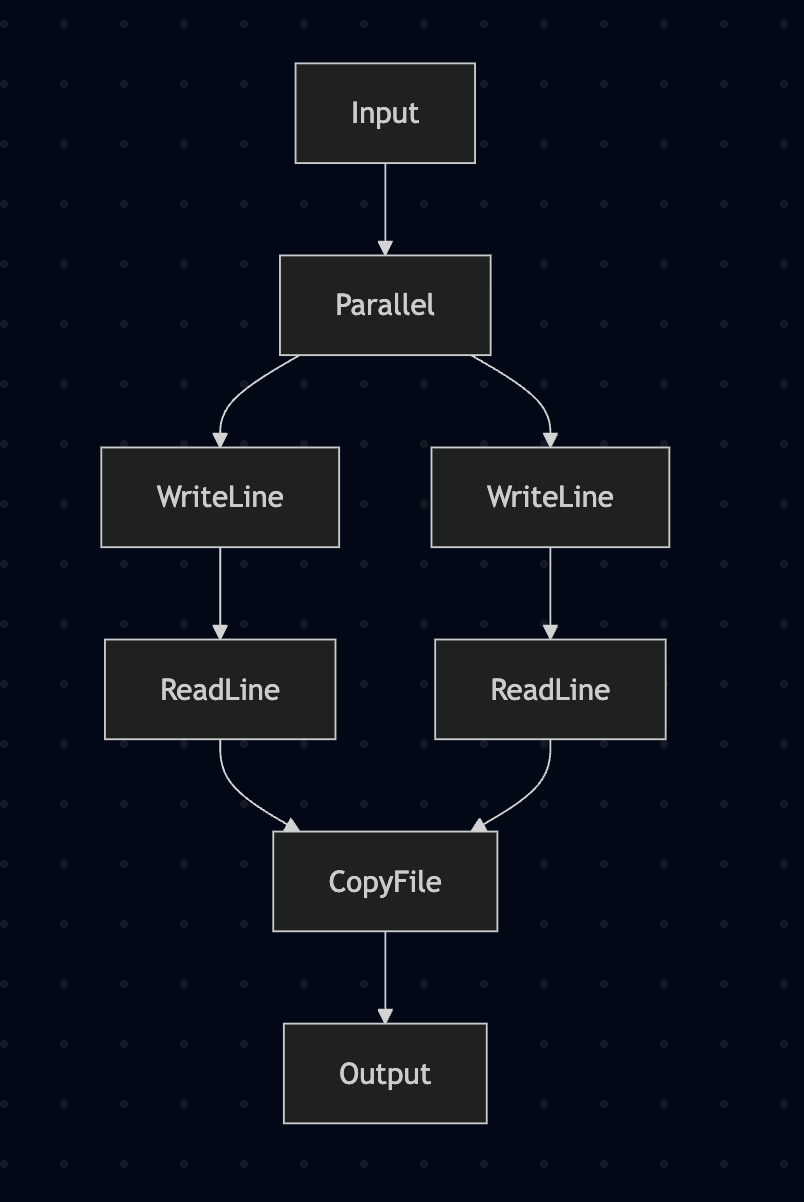
Here's what the diagram output for our fileCopyProgram looks like:

>>> diagram fileCopyProgram
flowchart TD
Input --> 0[Parallel]
0[Parallel] --> 1[WriteLine]
1[WriteLine] --> 2[ReadLine]
0[Parallel] --> 3[WriteLine]
3[WriteLine] --> 4[ReadLine]
2[ReadLine] --> 5[CopyFile]
4[ReadLine] --> 5[CopyFile]
5[CopyFile] --> Output

And rendered:

fileCopyProgram

Pretty cool eh?

Diagramming is just one thing you can do with our CommandTree, it's just data, you can fold over it to get all the effects, analyze which effects depend on which others, all sorts of things. This provides more clarity into what's happening than Selective's Over and Under newtypes.

This was a very simple example, but I promise you, with combinations of arr, (***) and first/second you can do any possible routing of values that you might like.

What you can't do yet, however, is to branch between possible execution paths, then run only one of them.

Let's add that.

Branching with ArrowChoice

Luckily for us, adding branching is pretty straight-forward. There's an aptly named ArrowChoice in base that we'll go ahead and implement.

ArrowChoice adds a new combinator:

(+++) :: ArrowChoice k => k a b -> k c d -> k (Either a c) (Either b d)

Similar to how (***) lets us represent two parallel and independent programs and fuse them into a single arrow which runs both, (+++) lets us introduce a conditional branch to our program, only one path will be executed based on whether the input value is a Left or a Right.

By implementing (+++) we also get the similar (|||) for free:

(|||) :: ArrowChoice k => k a c -> k b c -> k (Either a b) c

Let's add a Branch case to our CommandTree and implement ArrowChoice for our CommandRecorder.

data CommandTree eff
  = Effect eff
  | Identity
  | Composed (CommandTree eff {- >>> -}) (CommandTree eff)
  | Parallel
      (CommandTree eff) -- First
      (CommandTree eff) -- Second
  | Branch
      (CommandTree eff) -- Left
      (CommandTree eff) -- Right
  deriving (Show, Eq, Ord, Functor, Traversable, Foldable)

instance ArrowChoice (CommandRecorder eff) where
  (CommandRecorder cmds1) +++ (CommandRecorder cmds2) = CommandRecorder (Branch cmds1 cmds2)

No problem. As a reminder, here's the branching program we expressed using Selective Applicatives last time:

-- | A program using Selective effects
myProgram :: (ReadWriteDelete m) => m String
myProgram =
  let msgKind =
        Selective.matchS
          -- The list of values our program has explicit branches for.
          -- These are the values which will be used to crawl codepaths when
          -- analysing your program using `Over`.
          (Selective.cases ["friendly", "mean"])
          -- The action we run to get the input
          readLine
          -- What to do with each input
          ( \case
              "friendly" -> writeLine ("Hello! what is your name?") *> readLine
              "mean" ->
                let msg = unlines [ "Hey doofus, what do you want?"
                                  , "Too late. I deleted your hard-drive."
                                  , "How do you feel about that?"
                                  ]
                 in writeLine msg *> deleteMyHardDrive *> readLine
              -- This can't actually happen.
              _ -> error "impossible"
          )
      prompt = writeLine "Select your mood: friendly or mean"
      fallback =
        (writeLine "That was unexpected. You're an odd one aren't you?")
          <&> \() actualInput -> "Got unknown input: " <> actualInput
   in prompt
        *> Selective.branch
          msgKind
          fallback
          (pure id)

This example was always a bit forced just because of how limited Selective Applicatives are, but let's copy it over into our Arrow setup anyways.

First we'll implement ArrowChoice for our CommandRecorder.

-- Define our effects
class (Arrow k) => ReadWriteDelete k where
  readLine :: k () String

  writeLine :: k String ()

  deleteMyHardDrive :: k () ()

-- New commands for the new effects
data Command
  = ReadLine
  | WriteLine
  | DeleteMyHardDrive
  deriving (Show)

-- Track the effects
instance ReadWriteDelete CommandRecorder where
  readLine = CommandRecorder (Pure ReadLine)
  writeLine = CommandRecorder (Pure WriteLine)
  deleteMyHardDrive = CommandRecorder (Pure DeleteMyHardDrive)

-- Here's the runnable implementation
instance ReadWriteDelete (Kleisli IO) where
  readLine = Kleisli $ \() -> getLine
  writeLine = Kleisli $ \msg -> putStrLn msg
  deleteMyHardDrive = Kleisli $ \() -> putStrLn "Deleting hard drive... Just kidding!"

And here's our program which uses ArrowChoice:

branchingProgram :: (ReadWriteDelete k, ArrowChoice k) => k () ()
branchingProgram =
  pureC "Select your mood: friendly or mean"
    >>> writeLine
    >>> readLine
    >>> mapC
      ( \case
          "mean" -> Left ()
          "friendly" -> Right ()
          -- Just default to friendly
          _ -> Right ()
      )
    >>> let friendly =
              pureC "Hello! what is your name?"
                >>> writeLine
                >>> readLine
                >>> mapC (\name -> "Lovely to meet you, " <> name <> "!")
                >>> writeLine
            mean =
              pureC
                ( unlines
                    [ "Hey doofus, what do you want?",
                      "Too late. I deleted your hard-drive.",
                      "How do you feel about that?"
                    ]
                )
                >>> writeLine
                >>> deleteMyHardDrive
         in mean ||| friendly

Notice again, this version is actually more expressive than the Selective Applicative version, it actually greets the user by the name they provided, how kind.

I'll elide the edits to the mermaid renderer, Branch is very similar to the implementation of Parallel.

Let's make a mermaid chart like before:

>>> diagram branchingProgram
flowchart TD
Input --> 0[WriteLine]
0[WriteLine] --> 1[ReadLine]
1[ReadLine] --> 2[Branch]
2[Branch] --> 3[WriteLine]
3[WriteLine] --> 4[DeleteMyHardDrive]
2[Branch] --> 5[WriteLine]
5[WriteLine] --> 6[ReadLine]
6[ReadLine] --> 7[WriteLine]
4[DeleteMyHardDrive] --> Output
7[WriteLine] --> Output

Branching Program

See how it's now clear that the effects on one branch differ from another?

And of course we can run it just as you'd expect:

>>> run branchingProgram
Select your mood: friendly or mean
friendly
Hello! what is your name?
Joe
Lovely to meet you, Joe!

>>> run branchingProgram
Select your mood: friendly or mean
mean
Hey doofus, what do you want?
Too late. I deleted your hard-drive.
How do you feel about that?

Deleting hard drive... Just kidding!

Okay, so the syntax of that last example was starting to get pretty hairy, if only there was something like do-notation, but for arrows...

Arrow Notation

By enabling the {-# LANGUAGE Arrows #-} pragma we can use a form of do-notation with arrows. It will automatically route your inputs wherever you need them using combinators from the Arrow class and will even translate if and case statements into ArrowChoice combinators, it's very impressive.

I won't explain Arrow Notation deeply here, so go ahead and check out the GHC Manual for a more detailed look.

Here's what our branching program looks like when we translate it:

branchingProgramArrowNotation :: (ReadWriteDelete k, ArrowChoice k) => k () ()
branchingProgramArrowNotation = proc () -> do
  writeLine -< "Select your mood: friendly or mean"
  mood <- readLine -< ()
  case mood of
    "mean" -> mean -< ()
    "friendly" -> friendly -< ()
    _ -> friendly -< ()
  where
    friendly = proc () -> do
      writeLine -< "Hello! what is your name?"
      name <- readLine -< ()
      writeLine -< "Lovely to meet you, " <> name <> "!"

    mean = proc () -> do
      writeLine
        -<
          unlines
            [ "Hey doofus, what do you want?",
              "Too late. I deleted your hard-drive.",
              "How do you feel about that?"
            ]
      deleteMyHardDrive -< ()

It takes a bit of getting used to, but it's not so bad.

Here's the diagram, so we can get an idea of how it's being translated:

Arrow Notation Messy

It's not quite as pretty, the translation introduces a lot of unnecessary calls to Parallel where it's just inserting Identity on the other side, this is perfectly valid, since the Category laws require that the Identity won't affect behaviour, but in our case it's messy and is clogging up our diagram, so let's clean it up.

The command tree we build as an intermediate step is just a value, so we can transform it to clean it up no problem.

If you derive Data and Plated for our Command and CommandTree types then we can do this with a simple transform on the tree. transform will rebuild the tree from the bottom up removing any redundant Identity nodes as it goes.

unredundify :: (Data eff) => CommandTree eff -> CommandTree eff
unredundify = transform \case
  Parallel Identity right -> right
  Parallel left Identity -> left
  Composed Identity right -> right
  Composed left Identity -> left
  other -> other

Diagramming the unredundified version looks much cleaner:

Arrow Notation Cleaner

We can see here that the with multiple arms are getting collapsed into a sequence of binary branches, which is perfectly correct of course, but if you wanted to diagram it as a single branch you could rewrite the Branch constructor to have a list of options and collapse them all down with another rewrite rule. Same for Parallels of course. You can really do whatever is most useful for your use-case.

Arrow notation has its quirks, but it's still a substantial improvement over doing argument routing completely manually.

Static vs Dynamic data

It's worth a quick note on the difference between static and dynamic data with Arrows. With Applicatives, all the data needed to define an effect's behaviour was static, that is, it must be known at the time the program was constructed, though this might still be at runtime for the greater Haskell program.

With Arrows it's possible to interleave static and dynamic data, it's up to the author of the interface.

For example, if one were constructing a build-system they might have an interface like this:

class (Arrow k) => Builder k where
  dynamicReadFile :: k FilePath String
  staticReadFile :: FilePath -> k () String

dynamicReadFile takes its FilePath as a dynamic input, so we won't know which file we're going to read until execution time, however staticReadFile takes its FilePath as a static input. You pass it a single FilePath as a Haskell value when you construct the program. In this case we can embed the FilePath into the structure of the effect itself so that it's available during analysis.

While this is a bit more of an advanced use-case, it can be very useful. In the build-system case you could provide any statically known dependency files using staticReadFile and the build-system could check if those files have changed since the last run and safely replace some subtrees of the build with cached results if no dependencies in that subtree have changed.

This sort of thing takes careful thought and design, but provides a lot of flexibility which can unlock whole new programming techniques.

Folks may well have heard of Haxl, it's a Haskell library for analyzing programs and batching and caching requests to remote data sources. The implementation and interface for Haxl is moderately complex, and is limited in what it can do by the fact that it uses Monads. I'm curious how effective an Arrow-based version could be.

What's next?

We explored enough classes to enable most basic programs here. At this point you can branch, express independence between computations, and route input anywhere you need it. In case you're still hankering for a bit more expressive power we'll do a lightning quick tour of a few more classes.

There's ArrowLoop which encodes fixed-point style recursion.

class Arrow a => ArrowLoop a where
  loop :: a (b, d) (c, d) -> a b c

Interestingly, this is actually just another name for Costrong, as you can see by comparing with Costrong from the profunctors package.

If you really really need to be able to completely restructure your program on the fly you can do so using the ArrowApply class, which enables applying arbitrary runtime-created arrows.

class Arrow a => ArrowApply a where
    app :: a (a b c, b) c

This gives you the wildly expressive power to define entirely new code-paths at runtime. I'd still argue that reasonable programs that actually need to do this are pretty rare, but sometimes it's a useful shortcut to avoid some tedium. Note that if you use app, any effects within the dynamically applied arrow will be hidden from analysis, but you can still analyze the non-dynamic parts.

There are a few additional interesting classes which are strangely missing from base; but they have counterparts in profunctors. One example would be an arrow counterpart to Cochoice, which, if it existed, would look something like this:

class (Arrow k) => ArrowCochoice k where
  unright :: k (Either d a) (Either d b) -> k a b
  unleft :: k (Either a d) (Either b d) -> k a b

While the behaviour ultimately depends on the implementation, you can use this to implement things like recursive loops and while-loops, which avoids one of the more common needs for ArrowApply while preserving analysis over the contents of the loop.

There's some other good stuff in profunctors so I'd recommend just browsing around over there, (Thanks Ed). Traversing lets you apply a profunctor to elements of a Traversable container, Mapping does the same for Functors.

Anyways, you can see that most behaviours you take for granted when writing Haskell code with arbitrary functions in do-notation binds can generally be decomposed into some combination of Arrow typeclasses which accomplish the same thing. Using the principal of least-power is a good rule of thumb here. Generally you should use the lowest-power abstraction you can reasonably encode your program with, that will ensure you'll have the strongest potential for analysis.

In Summary

We've discovered that by switching from the Functor-Applicative-Monad effect system to a Category and Arrow hierarchy we can express significantly more complex and expressive programs while maintaining the ability to deeply introspect the programs we create.

We learned how we can collect additional typeclasses to gain more expressive power, and how we can implement custom instances to analyze and even diagram our programs.

Lastly we took a look at Arrow notation and how it improves the burden of syntax for writing these sorts of programs.

So, should we all abandon Monads and write everything using Arrows instead? Truthfully, I do believe they comprise a better foundation; so while the current Haskell ecosystem is all-in on Monads, if you the reader happen to be designing the effects system for a brand new functional programming language, why not give Arrows a try?

Hopefully you learned something 🤞! Did you know I'm currently writing a book? It's all about Lenses and Optics! It takes you all the way from beginner to optics-wizard and it's currently in early access! Consider supporting it, and more posts like this one by pledging on my Patreon page! It takes quite a bit of work to put these things together, if I managed to teach your something or even just entertain you for a minute or two maybe send a few bucks my way for a coffee? Cheers! �

Become a Patron!

October 16, 2025 12:00 AM

October 14, 2025

Sandy Maguire

Arrows to Arrows, Categories to Queries

I’ve had a little time off of work as of late, and been spending it in characteristically unwise ways. In particular, I’ve written a little programming language that compiles to SQL. I call it catlang. That’s not to say that I’ve written a new query language. It’s a programming language, whose compiler spits out one giant SELECT statement. When you run that query in postgres, you get the output of your program.

Why have I done this? Because I needed a funny compilation target to test out the actual features of the language, which is that its intermediary language is a bunch of abstract category theory nonsense. Which I’ll get to. But I’m sure you first want to see this bad boy in action.

Behold, the function that returns 100 regardless of what input you give it. But it does it with the equivalent of a while loop:

count : Int -> Int
count =
  x ->
    loop x
      i ->
        n <- join id id -< i
        z <- abs . (-) -< (n, 100)
        case z of
          inl _ -> inr . (+) -< (n, 1)
          inr _ -> inl -< n

If you’re familiar with arrow notation, you’ll notice the above looks kinda like one big proc block. This is not a coincidence (because nothing is a coincidence). I figured if I were to go through all of this work, we might as well get a working arrow desugarer out of the mix. But I digress; that’s a story for another time.

Anyway, what’s going on here is we have an arrow count, which takes a single argument x. We then loop, starting from the value of x. Inside the loop, we now have a new variable i, which we do some voodoo on to compute n—the current value of the loop variable. Then we subtract 100 from n, and take the absolute value. The abs function here is a bit odd; it returns Left (abs x) if the input was negative, and Right x otherwise. Then we branch on the output of abs, where Left and Right have been renamed inl and inr respectively. If n - 100 was less than zero, we find ourselves in the inl case, where we add 1 to n and wrap the whole thing in inr—which the loop interprets as “loop again with this new value.” Otherwise, n - 100 was non-negative, and so we can return n directly.

Is it roundabout? You bet! The obtuseness here is not directly a feature, I was just looking for conceptually simple things I could do which would be easy to desugar into category-theoretical stuff. Which brings us to the intermediary language. After desugaring the source syntax for count above, we’re left with this IL representation:

  id △ id
⨟ cochoice
    ( undist
    ⨟   ( (prj₁ ⨟ id ▽ id) △ id
          ⨟   ( prj₁ △ 100
              ⨟ (-)
              ⨟ abs
              )
            △ id
          ⨟ prj₁ △ id
          ⨟ dist
          ⨟   ( (prj₂ ⨟ prj₂ ⨟ prj₁) △ 1
              ⨟ (+)
              ⨟ inr
              )
            ▽ ( prj₂
              ⨟ prj₂
              ⨟ prj₁
              ⨟ inl
              )
        )
      △ prj₂
    ⨟ dist
    )
⨟ prj₁

We’ll discuss all of this momentarily, but for now, just let your eyes glaze over the pretty unicode.

The underlying idea here is that each of these remaining symbols has very simple and specific algebraic semantics. For example, A ⨟ B means “do A and pipe the result into B.” By giving a transformation from this categorical IL into other domains, it becomes trivial to compile catlang to all sorts of weird compilation targets. Like SQL.

You’re probably wondering what the generated SQL looks like. Take a peek if you dare.

Ungodly Compiled SQL
SELECT
f0 AS f0
FROM
(SELECT
 f0 AS f0, f1 AS f1
 FROM
 (SELECT *
  FROM
  (WITH t0 AS
   (SELECT *
    FROM
    (WITH RECURSIVE recursion AS
     (SELECT
      clock_timestamp() as step
      , *
      FROM
      (WITH t1 AS
       (SELECT *
        FROM
        (SELECT
         f0 AS f0, f1 AS f1, NULL::integer AS f2, NULL::integer AS f3
         FROM
         (WITH t2 AS
          (SELECT * FROM (SELECT 0 as f0) AS _)
          SELECT *
          FROM
          (SELECT * FROM (SELECT f0 AS f0 FROM t2 AS _) AS _
           CROSS JOIN
           (SELECT f0 AS f1 FROM t2 AS _))
          AS _)
         AS _)
        AS _)
       SELECT *
       FROM
       (WITH t3 AS
        (SELECT *
         FROM
         (-- undist
          SELECT *
          FROM
          (SELECT
           f0 AS f0, NULL::integer AS f1, f1 AS f2
           FROM
           (-- undist1
            SELECT * FROM t1 AS _ WHERE "f0" IS NOT NULL)
           AS _)
          AS _
          UNION
          SELECT *
          FROM
          (SELECT
           NULL::integer AS f0, f2 AS f1, f3 AS f2
           FROM
           (-- dist2
            SELECT * FROM t1 AS _ WHERE "f2" IS NOT NULL)
           AS _)
          AS _)
         AS _)
        SELECT *
        FROM
        (WITH t4 AS
         (SELECT *
          FROM
          (SELECT *
           FROM
           (SELECT
            f0 AS f0, f1 AS f1
            FROM
            (WITH t5 AS
             (SELECT * FROM t3 AS _)
             SELECT *
             FROM
             (WITH t6 AS
              (SELECT *
               FROM
               (SELECT *
                FROM
                (SELECT
                 f0 AS f0
                 FROM
                 (WITH t7 AS
                  (SELECT * FROM (SELECT f0 AS f0, f1 AS f1 FROM t5 AS _) AS _)
                  SELECT *
                  FROM
                  (SELECT *
                   FROM
                   (SELECT
                    f0 AS f0
                    FROM
                    (-- join1
                     SELECT * FROM t7 AS _ WHERE "f0" IS NOT NULL)
                    AS _)
                   AS _
                   UNION
                   SELECT *
                   FROM
                   (SELECT
                    f1 AS f0
                    FROM
                    (-- join2
                     SELECT * FROM t7 AS _ WHERE "f1" IS NOT NULL)
                    AS _)
                   AS _)
                  AS _)
                 AS _)
                AS _
                CROSS JOIN
                (SELECT f0 AS f1, f1 AS f2, f2 AS f3 FROM t5 AS _))
               AS _)
              SELECT *
              FROM
              (WITH t8 AS
               (SELECT *
                FROM
                (SELECT *
                 FROM
                 (SELECT
                  f0 AS f0, f1 AS f1
                  FROM
                  (WITH t9 AS
                   (SELECT *
                    FROM
                    (SELECT
                     f0 - f1 AS f0
                     FROM
                     (WITH t10 AS
                      (SELECT * FROM t6 AS _)
                      SELECT *
                      FROM
                      (SELECT *
                       FROM
                       (SELECT f0 AS f0 FROM (SELECT f0 AS f0 FROM t10 AS _) AS _)
                       AS _
                       CROSS JOIN
                       (SELECT f0 AS f1 FROM (SELECT 100 as f0 FROM t10 AS _) AS _))
                      AS _)
                     AS _)
                    AS _)
                   SELECT *
                   FROM
                   (SELECT *
                    FROM
                    (SELECT
                     abs(f0) as f0, NULL::integer as f1
                     FROM
                     t9
                     AS _
                     WHERE
                     f0 < 0)
                    AS _
                    UNION
                    SELECT *
                    FROM
                    (SELECT NULL::integer as f0, f0 as f1 FROM t9 AS _ WHERE f0 >= 0)
                    AS _)
                   AS _)
                  AS _)
                 AS _
                 CROSS JOIN
                 (SELECT f0 AS f2, f1 AS f3, f2 AS f4, f3 AS f5 FROM t6 AS _))
                AS _)
               SELECT *
               FROM
               (WITH t11 AS
                (SELECT *
                 FROM
                 (SELECT *
                  FROM
                  (SELECT
                   f0 AS f0, f1 AS f1
                   FROM
                   (SELECT f0 AS f0, f1 AS f1 FROM t8 AS _)
                   AS _)
                  AS _
                  CROSS JOIN
                  (SELECT
                   f0 AS f2, f1 AS f3, f2 AS f4, f3 AS f5, f4 AS f6, f5 AS f7
                   FROM
                   t8
                   AS _))
                 AS _)
                SELECT *
                FROM
                (WITH t12 AS
                 (SELECT *
                  FROM
                  (-- dist
                   SELECT *
                   FROM
                   (SELECT
                    f0 AS f0, f2 AS f1, NULL::integer AS f10, NULL::integer AS f11, NULL::integer AS f12, NULL::integer AS f13, f3 AS f2, f4 AS f3, f5 AS f4, f6 AS f5, f7 AS f6, NULL::integer AS f7, NULL::integer AS f8, NULL::integer AS f9
                    FROM
                    (-- dist1
                     SELECT * FROM t11 AS _ WHERE "f0" IS NOT NULL)
                    AS _)
                   AS _
                   UNION
                   SELECT *
                   FROM
                   (SELECT
                    NULL::integer AS f0, NULL::integer AS f1, f4 AS f10, f5 AS f11, f6 AS f12, f7 AS f13, NULL::integer AS f2, NULL::integer AS f3, NULL::integer AS f4, NULL::integer AS f5, NULL::integer AS f6, f1 AS f7, f2 AS f8, f3 AS f9
                    FROM
                    (-- dist2
                     SELECT * FROM t11 AS _ WHERE "f1" IS NOT NULL)
                    AS _)
                   AS _)
                  AS _)
                 SELECT *
                 FROM
                 (SELECT *
                  FROM
                  (SELECT
                   NULL::integer AS f0, f0 AS f1
                   FROM
                   (SELECT
                    f0 + f1 AS f0
                    FROM
                    (WITH t13 AS
                     (SELECT *
                      FROM
                      (SELECT
                       f0 AS f0, f1 AS f1, f2 AS f2, f3 AS f3, f4 AS f4, f5 AS f5, f6 AS f6
                       FROM
                       (-- join1
                        SELECT * FROM t12 AS _
                        WHERE
                        ("f0" IS NOT NULL) AND ((("f1" IS NOT NULL) OR ("f2" IS NOT NULL)) AND (("f3" IS NOT NULL) AND ((("f4" IS NOT NULL) OR ("f5" IS NOT NULL)) AND ("f6" IS NOT NULL)))))
                       AS _)
                      AS _)
                     SELECT *
                     FROM
                     (SELECT *
                      FROM
                      (SELECT
                       f0 AS f0
                       FROM
                       (SELECT
                        f0 AS f0
                        FROM
                        (SELECT
                         f2 AS f0, f3 AS f1, f4 AS f2, f5 AS f3
                         FROM
                         (SELECT
                          f1 AS f0, f2 AS f1, f3 AS f2, f4 AS f3, f5 AS f4, f6 AS f5
                          FROM
                          t13
                          AS _)
                         AS _)
                        AS _)
                       AS _)
                      AS _
                      CROSS JOIN
                      (SELECT f0 AS f1 FROM (SELECT 1 as f0 FROM t13 AS _) AS _))
                     AS _)
                    AS _)
                   AS _)
                  AS _
                  UNION
                  SELECT *
                  FROM
                  (SELECT
                   f0 AS f0, NULL::integer AS f1
                   FROM
                   (SELECT
                    f0 AS f0
                    FROM
                    (SELECT
                     f2 AS f0, f3 AS f1, f4 AS f2, f5 AS f3
                     FROM
                     (SELECT
                      f1 AS f0, f2 AS f1, f3 AS f2, f4 AS f3, f5 AS f4, f6 AS f5
                      FROM
                      (SELECT
                       f7 AS f0, f8 AS f1, f9 AS f2, f10 AS f3, f11 AS f4, f12 AS f5, f13 AS f6
                       FROM
                       (-- join2
                        SELECT * FROM t12 AS _
                        WHERE
                        ("f7" IS NOT NULL) AND ((("f8" IS NOT NULL) OR ("f9" IS NOT NULL)) AND (("f10" IS NOT NULL) AND ((("f11" IS NOT NULL) OR ("f12" IS NOT NULL)) AND ("f13" IS NOT NULL)))))
                       AS _)
                      AS _)
                     AS _)
                    AS _)
                   AS _)
                  AS _)
                 AS _)
                AS _)
               AS _)
              AS _)
             AS _)
            AS _)
           AS _
           CROSS JOIN
           (SELECT f0 AS f2 FROM (SELECT f2 AS f0 FROM t3 AS _) AS _))
          AS _)
         SELECT *
         FROM
         (-- dist
          SELECT *
          FROM
          (SELECT
           f0 AS f0, f2 AS f1, NULL::integer AS f2, NULL::integer AS f3
           FROM
           (-- dist1
            SELECT * FROM t4 AS _ WHERE "f0" IS NOT NULL)
           AS _)
          AS _
          UNION
          SELECT *
          FROM
          (SELECT
           NULL::integer AS f0, NULL::integer AS f1, f1 AS f2, f2 AS f3
           FROM
           (-- dist2
            SELECT * FROM t4 AS _ WHERE "f1" IS NOT NULL)
           AS _)
          AS _)
         AS _)
        AS _)
       AS _)
      AS _
      UNION ALL
      SELECT
      clock_timestamp() as step
      , *
      FROM
      (SELECT *
       FROM
       (WITH t14 AS
        (SELECT * FROM recursion AS _)
        SELECT *
        FROM
        (WITH t15 AS
         (SELECT *
          FROM
          (-- undist
           SELECT *
           FROM
           (SELECT
            f0 AS f0, NULL::integer AS f1, f1 AS f2
            FROM
            (-- undist1
             SELECT * FROM t14 AS _ WHERE "f0" IS NOT NULL)
            AS _)
           AS _
           UNION
           SELECT *
           FROM
           (SELECT
            NULL::integer AS f0, f2 AS f1, f3 AS f2
            FROM
            (-- dist2
             SELECT * FROM t14 AS _ WHERE "f2" IS NOT NULL)
            AS _)
           AS _)
          AS _)
         SELECT *
         FROM
         (WITH t16 AS
          (SELECT *
           FROM
           (SELECT *
            FROM
            (SELECT
             f0 AS f0, f1 AS f1
             FROM
             (WITH t17 AS
              (SELECT * FROM t15 AS _)
              SELECT *
              FROM
              (WITH t18 AS
               (SELECT *
                FROM
                (SELECT *
                 FROM
                 (SELECT
                  f0 AS f0
                  FROM
                  (WITH t19 AS
                   (SELECT * FROM (SELECT f0 AS f0, f1 AS f1 FROM t17 AS _) AS _)
                   SELECT *
                   FROM
                   (SELECT *
                    FROM
                    (SELECT
                     f0 AS f0
                     FROM
                     (-- join1
                      SELECT * FROM t19 AS _ WHERE "f0" IS NOT NULL)
                     AS _)
                    AS _
                    UNION
                    SELECT *
                    FROM
                    (SELECT
                     f1 AS f0
                     FROM
                     (-- join2
                      SELECT * FROM t19 AS _ WHERE "f1" IS NOT NULL)
                     AS _)
                    AS _)
                   AS _)
                  AS _)
                 AS _
                 CROSS JOIN
                 (SELECT f0 AS f1, f1 AS f2, f2 AS f3 FROM t17 AS _))
                AS _)
               SELECT *
               FROM
               (WITH t20 AS
                (SELECT *
                 FROM
                 (SELECT *
                  FROM
                  (SELECT
                   f0 AS f0, f1 AS f1
                   FROM
                   (WITH t21 AS
                    (SELECT *
                     FROM
                     (SELECT
                      f0 - f1 AS f0
                      FROM
                      (WITH t22 AS
                       (SELECT * FROM t18 AS _)
                       SELECT *
                       FROM
                       (SELECT *
                        FROM
                        (SELECT f0 AS f0 FROM (SELECT f0 AS f0 FROM t22 AS _) AS _)
                        AS _
                        CROSS JOIN
                        (SELECT f0 AS f1 FROM (SELECT 100 as f0 FROM t22 AS _) AS _))
                       AS _)
                      AS _)
                     AS _)
                    SELECT *
                    FROM
                    (SELECT *
                     FROM
                     (SELECT
                      abs(f0) as f0, NULL::integer as f1
                      FROM
                      t21
                      AS _
                      WHERE
                      f0 < 0)
                     AS _
                     UNION
                     SELECT *
                     FROM
                     (SELECT NULL::integer as f0, f0 as f1 FROM t21 AS _ WHERE f0 >= 0)
                     AS _)
                    AS _)
                   AS _)
                  AS _
                  CROSS JOIN
                  (SELECT f0 AS f2, f1 AS f3, f2 AS f4, f3 AS f5 FROM t18 AS _))
                 AS _)
                SELECT *
                FROM
                (WITH t23 AS
                 (SELECT *
                  FROM
                  (SELECT *
                   FROM
                   (SELECT
                    f0 AS f0, f1 AS f1
                    FROM
                    (SELECT f0 AS f0, f1 AS f1 FROM t20 AS _)
                    AS _)
                   AS _
                   CROSS JOIN
                   (SELECT
                    f0 AS f2, f1 AS f3, f2 AS f4, f3 AS f5, f4 AS f6, f5 AS f7
                    FROM
                    t20
                    AS _))
                  AS _)
                 SELECT *
                 FROM
                 (WITH t24 AS
                  (SELECT *
                   FROM
                   (-- dist
                    SELECT *
                    FROM
                    (SELECT
                     f0 AS f0, f2 AS f1, NULL::integer AS f10, NULL::integer AS f11, NULL::integer AS f12, NULL::integer AS f13, f3 AS f2, f4 AS f3, f5 AS f4, f6 AS f5, f7 AS f6, NULL::integer AS f7, NULL::integer AS f8, NULL::integer AS f9
                     FROM
                     (-- dist1
                      SELECT * FROM t23 AS _ WHERE "f0" IS NOT NULL)
                     AS _)
                    AS _
                    UNION
                    SELECT *
                    FROM
                    (SELECT
                     NULL::integer AS f0, NULL::integer AS f1, f4 AS f10, f5 AS f11, f6 AS f12, f7 AS f13, NULL::integer AS f2, NULL::integer AS f3, NULL::integer AS f4, NULL::integer AS f5, NULL::integer AS f6, f1 AS f7, f2 AS f8, f3 AS f9
                     FROM
                     (-- dist2
                      SELECT * FROM t23 AS _ WHERE "f1" IS NOT NULL)
                     AS _)
                    AS _)
                   AS _)
                  SELECT *
                  FROM
                  (SELECT *
                   FROM
                   (SELECT
                    NULL::integer AS f0, f0 AS f1
                    FROM
                    (SELECT
                     f0 + f1 AS f0
                     FROM
                     (WITH t25 AS
                      (SELECT *
                       FROM
                       (SELECT
                        f0 AS f0, f1 AS f1, f2 AS f2, f3 AS f3, f4 AS f4, f5 AS f5, f6 AS f6
                        FROM
                        (-- join1
                         SELECT * FROM t24 AS _
                         WHERE
                         ("f0" IS NOT NULL) AND ((("f1" IS NOT NULL) OR ("f2" IS NOT NULL)) AND (("f3" IS NOT NULL) AND ((("f4" IS NOT NULL) OR ("f5" IS NOT NULL)) AND ("f6" IS NOT NULL)))))
                        AS _)
                       AS _)
                      SELECT *
                      FROM
                      (SELECT *
                       FROM
                       (SELECT
                        f0 AS f0
                        FROM
                        (SELECT
                         f0 AS f0
                         FROM
                         (SELECT
                          f2 AS f0, f3 AS f1, f4 AS f2, f5 AS f3
                          FROM
                          (SELECT
                           f1 AS f0, f2 AS f1, f3 AS f2, f4 AS f3, f5 AS f4, f6 AS f5
                           FROM
                           t25
                           AS _)
                          AS _)
                         AS _)
                        AS _)
                       AS _
                       CROSS JOIN
                       (SELECT f0 AS f1 FROM (SELECT 1 as f0 FROM t25 AS _) AS _))
                      AS _)
                     AS _)
                    AS _)
                   AS _
                   UNION
                   SELECT *
                   FROM
                   (SELECT
                    f0 AS f0, NULL::integer AS f1
                    FROM
                    (SELECT
                     f0 AS f0
                     FROM
                     (SELECT
                      f2 AS f0, f3 AS f1, f4 AS f2, f5 AS f3
                      FROM
                      (SELECT
                       f1 AS f0, f2 AS f1, f3 AS f2, f4 AS f3, f5 AS f4, f6 AS f5
                       FROM
                       (SELECT
                        f7 AS f0, f8 AS f1, f9 AS f2, f10 AS f3, f11 AS f4, f12 AS f5, f13 AS f6
                        FROM
                        (-- join2
                         SELECT * FROM t24 AS _
                         WHERE
                         ("f7" IS NOT NULL) AND ((("f8" IS NOT NULL) OR ("f9" IS NOT NULL)) AND (("f10" IS NOT NULL) AND ((("f11" IS NOT NULL) OR ("f12" IS NOT NULL)) AND ("f13" IS NOT NULL)))))
                        AS _)
                       AS _)
                      AS _)
                     AS _)
                    AS _)
                   AS _)
                  AS _)
                 AS _)
                AS _)
               AS _)
              AS _)
             AS _)
            AS _
            CROSS JOIN
            (SELECT f0 AS f2 FROM (SELECT f2 AS f0 FROM t15 AS _) AS _))
           AS _)
          SELECT *
          FROM
          (-- dist
           SELECT *
           FROM
           (SELECT
            f0 AS f0, f2 AS f1, NULL::integer AS f2, NULL::integer AS f3
            FROM
            (-- dist1
             SELECT * FROM t16 AS _ WHERE "f0" IS NOT NULL)
            AS _)
           AS _
           UNION
           SELECT *
           FROM
           (SELECT
            NULL::integer AS f0, NULL::integer AS f1, f1 AS f2, f2 AS f3
            FROM
            (-- dist2
             SELECT * FROM t16 AS _ WHERE "f1" IS NOT NULL)
            AS _)
           AS _)
          AS _)
         AS _)
        AS _)
       AS _
       WHERE
       ("f2" IS NOT NULL) AND ("f3" IS NOT NULL))
      AS _)
     SELECT * FROM recursion ORDER BY step DESC LIMIT 1)
    AS _)
   SELECT *
   FROM
   (WITH t26 AS
    (SELECT *
     FROM
     (-- undist
      SELECT *
      FROM
      (SELECT
       f0 AS f0, NULL::integer AS f1, f1 AS f2
       FROM
       (-- undist1
        SELECT * FROM t0 AS _ WHERE "f0" IS NOT NULL)
       AS _)
      AS _
      UNION
      SELECT *
      FROM
      (SELECT
       NULL::integer AS f0, f2 AS f1, f3 AS f2
       FROM
       (-- dist2
        SELECT * FROM t0 AS _ WHERE "f2" IS NOT NULL)
       AS _)
      AS _)
     AS _)
    SELECT *
    FROM
    (WITH t27 AS
     (SELECT *
      FROM
      (SELECT *
       FROM
       (SELECT
        f0 AS f0, f1 AS f1
        FROM
        (WITH t28 AS
         (SELECT * FROM t26 AS _)
         SELECT *
         FROM
         (WITH t29 AS
          (SELECT *
           FROM
           (SELECT *
            FROM
            (SELECT
             f0 AS f0
             FROM
             (WITH t30 AS
              (SELECT * FROM (SELECT f0 AS f0, f1 AS f1 FROM t28 AS _) AS _)
              SELECT *
              FROM
              (SELECT *
               FROM
               (SELECT
                f0 AS f0
                FROM
                (-- join1
                 SELECT * FROM t30 AS _ WHERE "f0" IS NOT NULL)
                AS _)
               AS _
               UNION
               SELECT *
               FROM
               (SELECT
                f1 AS f0
                FROM
                (-- join2
                 SELECT * FROM t30 AS _ WHERE "f1" IS NOT NULL)
                AS _)
               AS _)
              AS _)
             AS _)
            AS _
            CROSS JOIN
            (SELECT f0 AS f1, f1 AS f2, f2 AS f3 FROM t28 AS _))
           AS _)
          SELECT *
          FROM
          (WITH t31 AS
           (SELECT *
            FROM
            (SELECT *
             FROM
             (SELECT
              f0 AS f0, f1 AS f1
              FROM
              (WITH t32 AS
               (SELECT *
                FROM
                (SELECT
                 f0 - f1 AS f0
                 FROM
                 (WITH t33 AS
                  (SELECT * FROM t29 AS _)
                  SELECT *
                  FROM
                  (SELECT *
                   FROM
                   (SELECT f0 AS f0 FROM (SELECT f0 AS f0 FROM t33 AS _) AS _)
                   AS _
                   CROSS JOIN
                   (SELECT f0 AS f1 FROM (SELECT 100 as f0 FROM t33 AS _) AS _))
                  AS _)
                 AS _)
                AS _)
               SELECT *
               FROM
               (SELECT *
                FROM
                (SELECT
                 abs(f0) as f0, NULL::integer as f1
                 FROM
                 t32
                 AS _
                 WHERE
                 f0 < 0)
                AS _
                UNION
                SELECT *
                FROM
                (SELECT NULL::integer as f0, f0 as f1 FROM t32 AS _ WHERE f0 >= 0)
                AS _)
               AS _)
              AS _)
             AS _
             CROSS JOIN
             (SELECT f0 AS f2, f1 AS f3, f2 AS f4, f3 AS f5 FROM t29 AS _))
            AS _)
           SELECT *
           FROM
           (WITH t34 AS
            (SELECT *
             FROM
             (SELECT *
              FROM
              (SELECT
               f0 AS f0, f1 AS f1
               FROM
               (SELECT f0 AS f0, f1 AS f1 FROM t31 AS _)
               AS _)
              AS _
              CROSS JOIN
              (SELECT
               f0 AS f2, f1 AS f3, f2 AS f4, f3 AS f5, f4 AS f6, f5 AS f7
               FROM
               t31
               AS _))
             AS _)
            SELECT *
            FROM
            (WITH t35 AS
             (SELECT *
              FROM
              (-- dist
               SELECT *
               FROM
               (SELECT
                f0 AS f0, f2 AS f1, NULL::integer AS f10, NULL::integer AS f11, NULL::integer AS f12, NULL::integer AS f13, f3 AS f2, f4 AS f3, f5 AS f4, f6 AS f5, f7 AS f6, NULL::integer AS f7, NULL::integer AS f8, NULL::integer AS f9
                FROM
                (-- dist1
                 SELECT * FROM t34 AS _ WHERE "f0" IS NOT NULL)
                AS _)
               AS _
               UNION
               SELECT *
               FROM
               (SELECT
                NULL::integer AS f0, NULL::integer AS f1, f4 AS f10, f5 AS f11, f6 AS f12, f7 AS f13, NULL::integer AS f2, NULL::integer AS f3, NULL::integer AS f4, NULL::integer AS f5, NULL::integer AS f6, f1 AS f7, f2 AS f8, f3 AS f9
                FROM
                (-- dist2
                 SELECT * FROM t34 AS _ WHERE "f1" IS NOT NULL)
                AS _)
               AS _)
              AS _)
             SELECT *
             FROM
             (SELECT *
              FROM
              (SELECT
               NULL::integer AS f0, f0 AS f1
               FROM
               (SELECT
                f0 + f1 AS f0
                FROM
                (WITH t36 AS
                 (SELECT *
                  FROM
                  (SELECT
                   f0 AS f0, f1 AS f1, f2 AS f2, f3 AS f3, f4 AS f4, f5 AS f5, f6 AS f6
                   FROM
                   (-- join1
                    SELECT * FROM t35 AS _
                    WHERE
                    ("f0" IS NOT NULL) AND ((("f1" IS NOT NULL) OR ("f2" IS NOT NULL)) AND (("f3" IS NOT NULL) AND ((("f4" IS NOT NULL) OR ("f5" IS NOT NULL)) AND ("f6" IS NOT NULL)))))
                   AS _)
                  AS _)
                 SELECT *
                 FROM
                 (SELECT *
                  FROM
                  (SELECT
                   f0 AS f0
                   FROM
                   (SELECT
                    f0 AS f0
                    FROM
                    (SELECT
                     f2 AS f0, f3 AS f1, f4 AS f2, f5 AS f3
                     FROM
                     (SELECT
                      f1 AS f0, f2 AS f1, f3 AS f2, f4 AS f3, f5 AS f4, f6 AS f5
                      FROM
                      t36
                      AS _)
                     AS _)
                    AS _)
                   AS _)
                  AS _
                  CROSS JOIN
                  (SELECT f0 AS f1 FROM (SELECT 1 as f0 FROM t36 AS _) AS _))
                 AS _)
                AS _)
               AS _)
              AS _
              UNION
              SELECT *
              FROM
              (SELECT
               f0 AS f0, NULL::integer AS f1
               FROM
               (SELECT
                f0 AS f0
                FROM
                (SELECT
                 f2 AS f0, f3 AS f1, f4 AS f2, f5 AS f3
                 FROM
                 (SELECT
                  f1 AS f0, f2 AS f1, f3 AS f2, f4 AS f3, f5 AS f4, f6 AS f5
                  FROM
                  (SELECT
                   f7 AS f0, f8 AS f1, f9 AS f2, f10 AS f3, f11 AS f4, f12 AS f5, f13 AS f6
                   FROM
                   (-- join2
                    SELECT * FROM t35 AS _
                    WHERE
                    ("f7" IS NOT NULL) AND ((("f8" IS NOT NULL) OR ("f9" IS NOT NULL)) AND (("f10" IS NOT NULL) AND ((("f11" IS NOT NULL) OR ("f12" IS NOT NULL)) AND ("f13" IS NOT NULL)))))
                   AS _)
                  AS _)
                 AS _)
                AS _)
               AS _)
              AS _)
             AS _)
            AS _)
           AS _)
          AS _)
         AS _)
        AS _)
       AS _
       CROSS JOIN
       (SELECT f0 AS f2 FROM (SELECT f2 AS f0 FROM t26 AS _) AS _))
      AS _)
     SELECT *
     FROM
     (-- dist
      SELECT *
      FROM
      (SELECT
       f0 AS f0, f2 AS f1, NULL::integer AS f2, NULL::integer AS f3
       FROM
       (-- dist1
        SELECT * FROM t27 AS _ WHERE "f0" IS NOT NULL)
       AS _)
      AS _
      UNION
      SELECT *
      FROM
      (SELECT
       NULL::integer AS f0, NULL::integer AS f1, f1 AS f2, f2 AS f3
       FROM
       (-- dist2
        SELECT * FROM t27 AS _ WHERE "f1" IS NOT NULL)
       AS _)
      AS _)
     AS _)
    AS _)
   AS _)
  AS _
  WHERE
  ("f0" IS NOT NULL) AND ("f1" IS NOT NULL))
 AS _)
AS _;

It’s not pretty, rather amazingly, running the above query in postgres 17 will in fact return a single row with a single column whose value is 100. And you’d better believe it does it by actually looping its way up to 100. If you don’t believe me, make the following change:

-     SELECT * FROM recursion ORDER BY step DESC LIMIT 1)
+     SELECT * FROM recursion ORDER BY step DESC)

which will instead return a row for each step of the iteration.

There are some obvious optimizations I could make to the generated SQL, but it didn’t seem worth my time, since that’s not the interesting part of the project.

What the Hell Is Going On?

Let’s take some time to discuss the underlying category theory here. I am by no means an expert, but what I have learned after a decade of bashing my head against this stuff is that a little goes a long way.

For our intents and purposes, we have types, and arrows (functions) between types. We always have the identity “do nothing arrow” id:

id  :: a ~> a

and we can compose arrows by lining up one end to another:1

(⨟) :: (a ~> b) -> (b ~> c) -> (a ~> c)

Unlike Haskell (or really any programming language, for that matter), we DO NOT have the notion of function application. That is, there is no arrow:

-- doesn't exist!
($) :: (a ~> b) -> a -> b

You can only compose arrows, you can’t apply them. That’s why we call these things “arrows” rather than “functions.”

There are a bundle of arrows for working with product types. The two projection functions correspond to fst and snd, taking individual components out of pairs:

prj₁ :: (a, b) ~> a
prj₂ :: (a, b) ~> b

How do we get things into pairs in the first place? We can use the “fork” operation, which takes two arrows computing b and c, and generates a new arrow which generates a pair of (b, c):

(△)  :: (a ~> b) -> (a ~> c) -> (a ~> (b, c))

If you’re coming from a Haskell background, it’s tempting to think of this operation merely as the (,) pair constructor. But you’ll notice from the type of the computation that there can be no data dependency between b and c, thus we are free to parallelize each side of the pair.

In category theory, the distinction between left and right sides of an arrow is rather arbitrary. This gives rise to a notion called duality where we can flip the arrows around, and get cool new behavior. If we dualize all of our product machinery, we get the coproduct machinery, where a coproduct of a and b is “either a or b, but definitely not both nor neither.”

Swapping the arrow direction of prj₁ and prj₂, and replacing (,) with Either gives us the following injections:

inl :: a ~> Either a b
inr :: b ~> Either a b

and the following “join” operation for eliminating coproducts:

(▽) :: (a ~> c) -> (b ~> c) -> (Either a b ~> c)

Again, coming from Haskell this is just the standard either function. It corresponds to a branch between one of two cases.

As you can see, with just these eight operations, we already have a tremendous amount of expressivity. We can express data dependencies via and branching via . With we automatically encode opportunities for parallelism, and gain the ability to build complicated data structures, with prj₁ and prj₂ allowing us to get the information back out of the data structures.

You’ll notice in the IL that there are no variable names anywhere to be found. The desugaring of the source language builds a stack (via the something to allocate △ id pattern), and replaces subsequent variable lookups with a series of projections on the stack to find the value again. On one hand, this makes the categorical IL rather hard to read, but it makes it very easy to re-target! Many domains do have a notion of grouping, but don’t have a native notion of naming.

For example, in an electronic circuit, I can have a ribbon of 32 wires which represents an Int32. If I have another ribbon of 32 wires, I can trivially route both wires into a 64-wire ribbon corresponding to a pair of (Int32, Int32).

By eliminating names before we get to the IL, it means no compiler backend ever needs to deal with names. They can just work on a stack representation, and are free to special-case optimize series of projections if they are able to.

Of particular interest to this discussion is how we desugar loops in catlang. The underlying primitive is cochoice:

cochoice :: (Either a c ~> Either b c) -> (a ~> b)

which magically turns an arrow on Eithers into an arrow without the eithers. We obviously must run that arrow on eithers. If that function returns inl, then we’re happy and we can just output that. But if the function returns inr, we have no choice but to pass it back in to the eithered arrow. In Haskell, cochoice is implemented as:

cochoiceHask :: (Either a c -> Either b c) -> a -> c
cochoiceHask f = go . Left
  where
    go :: Either a c -> b
    go eac =
      case f eac of
        Left b -> b
        Right c -> go (Right c)

which as you can see, will loop until f finally returns a Left. What’s neat about this formulation of a loop is that we can statically differentiate between our first and subsequent passes through the loop body. The first time through eac is Left, while for all other times it is Right. We don’t take advantage of it in the original count program, but how many times have you written loop code that needs to initialize something its first time through?

Compiling to SQL

So that’s the underlying theory behind the IL. How can we compile this to SQL now?

As alluded to before, we simply need to give SQL implementations for each of the operations in the intermediary language. As a simple example, id compiles to SELECT * FROM {}, where {} is the input of the arrow.

The hardest part here was working out a data representation. It seems obvious to encode each element of a product as a new column, but what do we do about coproducts? After much work thought, I decided to flatten out the coproducts. So, for example, the type:

(Int, Either Int Int)

would be represented as three columns:

( f1 INT NOT NULL
, f2 INT
, f3 INT
)

with the constraint that exactly one of f2 or f3 would be IS NOT NULL at any given point in time.

With this hammered out, almost everything else is pretty trivial. Composition corresponds to a nested query. Forks are CROSS JOINs which concatenate the columns of each sub-query. Joins are UNIONs, where we add a WHERE field IS NOT NULL clause to enforce we’re looking at the correct coproduct constructor.

Cochoice is the only really tricky thing, but it corresponds to a recursive CTE. Generating a recursive CTE table for the computation isn’t too hard, but getting the final value out of it was surprisingly tricky. The semantics of SQL tables is that they are multisets and come with an arbitrary greatest element. Which is to say, you need an column structured in a relevant way in order to query the final result. Due to some quirks in what postgres accepts, and in how I structured my queries, it was prohibitively hard to insert a “how many times have I looped” column and order by that. So instead I cheated and added a clock_timestamp() as step column which looks at the processor clock and ordered by that.

This is clearly a hack, and presumably will cause problems if I ever add some primitives which generate more than one row, but again, this is just for fun and who cares. Send me a pull request if you’re offended by my chicanery!

Stupid Directions To Go In the Future

I’ve run out of vacation time to work on this project, so I’m probably not going to get around to the meta-circular stupidity I was planning.

The compiler still needs a few string-crunching primitives (which are easy to add), but then it would be simple to write a little brainfuck interpreter in catlang. Which I could then compile to SQL. Now we’ve got a brainfuck interpreter running in postgres. Of course, this has been done by hand before, but to my knowledge, never via compilation.

There exist C to brainfuck compilers. And postgres is written in C. So in a move that would make Xzibit proud, we could run postgres in postgres. And of course, it would be fun to run brainfuck in brainfuck. That’d be a cool catlang backend if someone wanted to contribute such a thing.

Notes and Due Diligence and What Have You

I am not the first person to do anything like this. The source language of catlang is heavily inspired by Haskell’s arrow syntax, which in turn is essentially a desugaring algorithm for Arrows. Arrows are slightly the wrong abstraction because they require an operation arr :: (a -> b) -> (a ~> b)—which requires you to be able to embed Haskell functions in your category, something which is almost never possible.

Unfortunately, arrow syntax in Haskell desugars down to arr for almost everything it does, which in turn makes arrow notation effectively useless. In an ideal world, everything I described in this blog post would be a tiny little Haskell library, with arrow notation doing the heavy lifting. But that is just not the world we live in.

Nor am I the first person to notice that there are categorical semantics behind programming languages. I don’t actually know whom to cite on this one, but it is well-established folklore that the lambda calculus corresponds to cartesian-closed categories. The “closed” part of “cartesian-closed” means we have an operation eval :: (a ~> b, a) ~> b, but everyone and their dog has implemented the lambda calculus, so I thought it would be fun to see how far we can get without it. This is not a limitation on catlang’s turing completeness (since cochoice gives us everything we need.)

I’ve been thinking about writing a category-first programming language for the better part of a decade, ever since I read Compiling to Categories. That paper takes Haskell and desugars it back down to categories. I stole many of the tricks here from that paper.

Anyway. All of the code is available on github if you’re interested in taking a look. The repo isn’t up to my usual coding standards, for which you have my apologies. Of note is the template-haskell backend which can spit out Haskell code; meaning it wouldn’t be very hard to make a quasiquoter to compile catlang into what Haskell’s arrow desugaring ought to be. If there’s enough clamor for such a thing, I’ll see about turning this part into a library.


  1. When looking at the types of arrows in this essay, we make the distinction that ~> are arrows that we can write in catlang, while -> exist in the metatheory.↩︎

October 14, 2025 02:31 PM

October 13, 2025

Monday Morning Haskell

Making Change: Array-Based DP

Today we’ll continue the study of Dynamic Programming we started last week. Last week’s problem let us use a very compact memory footprint, only remember a couple prior values. This week, we’ll study a very canonical DP problem that really forces us to store a longer array of prior values to help us populate the new solutions.

For an in-depth study of Dynamic Programming in Haskell and many other problem solving techniques, take a look at our Solve.hs course today! Module 3 focuses on algorithms, and introduces several steps leading up to understanding DP.

The Problem

Our problem today is Coin Change, and it’s relatively straightforward. We are given a list of coin values, and an amount to make change for. We want to find the smallest number of coins we can use to provide the given amount (or -1 if the amount cannot be made from the coins we have).

So for example, if we have coins [1,2,5], and we are trying to make 11 cents of change, the answer is 3 coins, because we take 2 5 coins and 1 1 coin.

If we have the coins [2,10,15] and the amount is 13, we should return -1, since there is no way to make 13 cents from these coins.

The Algorithm

Let us first observe that a greedy algorithm does not work here! We can’t simply take the largest coin under the remaining amount and then recurse. If we have coins like [1, 20, 25] and the amount is 40, we can do this with 2 coins (both 20), but taking a 25 coin to start is suboptimal.

The way we will do this is to build a DP array so that index i represents the fewest coins necessary to produce the amount i. All values are initially -1, to indicate that we might not be able to satisfy the number. However, we can set the index 0 as 0, since no coins are needed to give 0 cents.

So we have our base case, but how do we fill in index i, assuming we’ve filled in everything up to i - 1? The answer is that we will consider each coin we can use, and look back in the array based on its value. So if 5 is one of our coins, we’ll consider just adding 1 to the value at index i - 5. We’ll take the minimum value based on looking at all the different coin options, being careful to observe edge cases where no values are possible.

Unlike the last problem, this does require us to keep a larger array of values. We’re not just reaching back for the prior value in our array, we’re considering values that are much further back. Plus the amount of look-back we need is dynamic depending on the problem inputs.

We’ll write a solution where the array has size equal to the given amount (plus 1). It would be possible to instead use a structure whose size simply covers the range of possible coin values, but this becomes considerably more difficult.

Rust Solution

We’ll start with the Rust solution, since modifying arrays is more natural in Rust. What is unnatural in Rust is mixing integer types. Everything has to be usize if we’re going to index into arrays with it, so let’s start by converting the amount and the coins into usize:

```rust
pub fn coin_change(coins: Vec<i32>, amount: i32) -> i32 {
    let n = amount as usize;
    let cs: Vec<usize> = coins.into_iter().map(|x| x as usize).collect();
    ...
}

Now we’ll initialize our dp array. It should have a size equal to the amount plus 1 (we want indices 0 and amount to be valid). Most cells should initially be -1, but we’ll make the 0 index equal to 0 as our base case (no coins to make 0 cents of change). We’ll also return the final value from this array as our answer.

pub fn coin_change(coins: Vec<i32>, amount: i32) -> i32 {
    let n = amount as usize;
    let cs: Vec<usize> = coins.into_iter().map(|x| x as usize).collect();
    let mut dp = Vec::with_capacity(n + 1);
    dp.resize(n + 1, -1);
    dp[0] = 0;
    ...
    return dp[n];
}

Let’s set up our loops. We go through all the indices from 1 to amount, and loop through all the coins for each index.

pub fn coin_change(coins: Vec<i32>, amount: i32) -> i32 {
    let n = amount as usize;
    let cs: Vec<usize> = coins.into_iter().map(|x| x as usize).collect();
    let mut dp = Vec::with_capacity(n + 1);
    dp.resize(n + 1, -1);
    dp[0] = 0;
    for i in 1..=n {
        for coin in &cs {
            ...
        }
    }
    return dp[n];
}

Now let’s apply some rules for dealing with each coin. First, if the coin is larger than the index, we do nothing, since we can’t use it for this amount. Otherwise, we try to use it. We get a “previous” value for this coin, meaning we look at our dp table going back the number of spaces corresponding to the coin’s value.

pub fn coin_change(coins: Vec<i32>, amount: i32) -> i32 {
    ...
    for i in 1..=n {
        for coin in &cs {
            if *coin <= i {
                let prev = dp[i - coin];
                ...
            }
        }
    }
    return dp[n];
}

If the prior value is -1, we can ignore it. This means we can’t actually use this coin to form the value at this index. Otherwise, we look at the current value in the dp table for this index. We may have a value here from previous coins already. If this value is not -1, and it is larger than the value we get from using this new coin, we replace the value in the dp table:

pub fn coin_change(coins: Vec<i32>, amount: i32) -> i32 {
    let n = amount as usize;
    let cs: Vec<usize> = coins.into_iter().map(|x| x as usize).collect();
    let mut dp = Vec::with_capacity(n + 1);
    dp.resize(n + 1, -1);
    dp[0] = 0;
    for i in 1..=n {
        for coin in &cs {
            if *coin <= i {
                let prev = dp[i - coin];
                if prev != -1 && (dp[i] == -1 || prev + 1 < dp[i]) {
                    dp[i] = prev + 1;
                }
            }
        }
    }
    return dp[n];
}

And this completes our solution!

Haskell Solution

In Haskell, immutability makes DP with arrays a bit more challenging. We could use mutable arrays, but these are a little tricky (you can learn about them in Solve.hs).

Instead we’ll learn on the IntMap type, which is just like Data.Map but always uses Int for keys. This structure is “mutable” in the same way as other map-like structures in Haskell. We’ll write a core loop that takes this map as its stateful input, as well as the index:

import qualified Data.IntMap.Lazy as IM

coinChange :: [Int] -> Int -> Int
coinChange coins amount = ...
  where
    loop :: IM.IntMap Int -> Int -> Int
    loop dp i = ...

A notable difference with how we’ll use our map is that we don’t have entries for invalid indices. These will be absent, and we’ll use fromMaybe with our map to consider that they might not exist. As a first example of this, let’s do the base case for our loop. Once the index i exceeds our amount, we’ll return the value in our map at amount, or -1 if it doesn’t exist:

coinChange :: [Int] -> Int -> Int
coinChange coins amount = ...
  where
    loop :: IM.IntMap Int -> Int -> Int
    loop dp i = if i > amount then fromMaybe (-1) (IM.lookup amount dp)
      else ...

Now we need to loop through the coins while updating our IntMap. Hopefully you can guess what’s coming. We need to define a function that ends with a -> b -> b, where a is the new coin we’re processing and b is the IntMap. Then we can loop through the coins with foldr. This function will also take our current index, which will be constant across the loop of coins:

coinChange :: [Int] -> Int -> Int
coinChange coins amount = ...
  where
    coinLoop :: Int -> Int -> IM.IntMap Int -> IM.IntMap Int
    coinLoop i coin dp = ...

    loop :: IM.IntMap Int -> Int -> Int
    loop dp i = if i > amount then fromMaybe (-1) (IM.lookup amount dp)
      else ...

We consider the “previous” value, which we call -1 if it doesn’t exist. We also consider the “current” value for index i, but we use maxBound if it doesn’t exist. This is because we want to insert a new number if it’s smaller, and maxBound will always be larger:

coinChange :: [Int] -> Int -> Int
coinChange coins amount = ...
  where
    coinLoop :: Int -> Int -> IM.IntMap Int -> IM.IntMap Int
    coinLoop i coin dp =
      let prev = fromMaybe (-1) (IM.lookup (i - coin) dp)
          current = fromMaybe maxBound (IM.lookup i dp)
      in  ...

If the prior value doesn’t exist, or if the existing value is smaller than using the previous value (plus 1), then we keep dp the same. Otherwise we insert the new value at this index:

coinChange :: [Int] -> Int -> Int
coinChange coins amount = ...
  where
    coinLoop :: Int -> Int -> IM.IntMap Int -> IM.IntMap Int
    coinLoop i coin dp =
      let prev = fromMaybe (-1) (IM.lookup (i - coin) dp)
          current = fromMaybe maxBound (IM.lookup i dp)
      in  if prev == (-1) || current < prev + 1 then dp
            else IM.insert i (prev + 1) dp

    loop :: IM.IntMap Int -> Int -> Int
    loop dp i = if i > amount then fromMaybe (-1) (IM.lookup amount dp)
      else ...

Now to complete our function, we just have to invoke these two loops. The primary loop we invoke with a base map assigning 0 to 0. The secondary loop relies on foldr and looping over the coins. We use this result in our recursive call:

coinChange :: [Int] -> Int -> Int
coinChange coins amount = loop (IM.singleton 0 0) 1
  where
    coinLoop :: Int -> Int -> IM.IntMap Int -> IM.IntMap Int
    coinLoop i coin dp =
      let prev = fromMaybe (-1) (IM.lookup (i - coin) dp)
          current = fromMaybe maxBound (IM.lookup i dp)
      in  if prev == (-1) || current < prev + 1 then dp
            else IM.insert i (prev + 1) dp

    loop :: IM.IntMap Int -> Int -> Int
    loop dp i = if i > amount then fromMaybe (-1) (IM.lookup amount dp)
      else loop (foldr (coinLoop i) dp coins) (i + 1)

And now we’re done!

Conclusion

Our first two problems have been simple, 1-dimensional DP problems. But DP really shines as a technique when applied across multiple dimensions. In the next two weeks we’ll consider some of these multi-dimensional DP problems.

For more practice with DP and other algorithms, sign up for Solve.hs, our Haskell problem solving course! The course has hundreds of practice problems so you can hone your Haskell skills!

by James Bowen at October 13, 2025 08:30 AM

Well-Typed.Com

Verifying and testing timeliness constraints with io-sim

Testing and verifying concurrent systems is hard due to their non-deterministic nature — verifying behavior that changes with each execution is difficult. Race conditions thrive in the non-deterministic world of thread scheduling. Even more challenging is verifying timeliness constraints, i.e. ensuring that operations complete within specified deadlines or that service guarantees are maintained under load. Traditional testing approaches struggle with concurrency, and mocking strategies often fail to capture the subtle interactions between threads, time, and shared state that cause real production failures.

The io-sim Haskell library, developed by Well-Typed in partnership with engineers from IOG and Quviq, offers a compelling solution to this problem. The library provides a pure simulation environment for IO computations, enabling deterministic execution of concurrent code with accurate time simulation and detailed execution traces. Unlike other testing approaches, with io-sim one is able to write highly concurrent, real-time systems and verify their timeliness constraints in a deterministic manner, by accurately simulating GHC’s runtime system (e.g. asynchronous exceptions, timeouts & delays, etc.).

This blog post introduces and explores io-sim through a practical example: debugging an elevator controller that violates its response time requirements.

There’s also this great blog post announcing io-sim and it goes a bit more into detail about its features!

The Problem

Consider a simple elevator located in a three-floor building (ground, first , second). It takes roughly 1 second for the elevator to go up and down between each floor. The service requirement is: no passenger should wait more than 4 seconds from pressing the call button until the elevator doors open at their floor. It should be possible to test and verify this requirement when writing our elevator controller.

This ensures a reasonable quality of service and prevents frustration. Given the short distance between floors, 4 seconds is sensible. In the worst case, the elevator must travel from ground to second floor and back again.

Here’s a first attempt at modelling the system. Let’s start with the core data structures:

data Direction = Up | Down | None
  deriving (Eq, Show)

data Floor = Ground | First | Second
  deriving (Eq, Ord, Show, Enum)

data ElevatorState = ElevatorState
  { currentFloor :: Floor
  , moving       :: Direction
  , requests     :: [Floor]
  } deriving (Show)

The elevator’s state tracks three things: where it currently is, which direction it’s moving (if any), and a queue of floor requests.

The system has two main components that run concurrently:

  • An elevator controller that continuously processes the request queue
  • Button press handler that adds new floor requests

Let’s look at the controller first:

-- | Initialize an empty elevator state.
--
-- The elevator starts on the ground floor
--
initElevator :: IO (TVar ElevatorState)
initElevator = newTVarIO $ ElevatorState Ground None []

-- | Elevator controller logic.
--
-- 1. Read the current 'ElevatorState'
-- 2. Check if there are any requested floors
-- 3.
--    3.1. Block waiting for new requests if there aren't any
--    3.2. If there any requests, move to the floor at the top of the queue.
--
-- Straightforward FIFO elevator algorithm.
--
elevatorController :: TVar ElevatorState -> IO ()
elevatorController elevatorVar = forever $ do
  -- Atomically get the next floor from the queue
  (nextFloor, dir) <- atomically $ do
    state <- readTVar elevatorVar
    case requests state of
      []               -> retry  -- Block until a request arrives
      (targetFloor:rs) -> do
        -- Remove the floor from queue and start moving
        let direction = getDirection (currentFloor state) targetFloor
        writeTVar elevatorVar $ state
          { moving = direction, requests = rs }
        return (targetFloor, direction)

  putStrLn ("Going " ++ show dir ++ " to " ++ show nextFloor)
  moveToFloor elevatorVar nextFloor

The moveToFloor function simulates the physical movement of the elevator.

moveToFloor :: TVar ElevatorState -> Floor -> IO ()
moveToFloor elevatorVar targetFloor = do
  elevatorState <- readTVarIO elevatorVar
  when (currentFloor elevatorState /= targetFloor) $ do
    -- Takes 1 second to move between floors
    threadDelay (1000000 * numberOfFloorsToMove)
    atomically $
      modifyTVar elevatorVar (\elevatorState' ->
        elevatorState' { currentFloor = targetFloor
                       , moving       = Idle
                       }
        )
  putStrLn ("Arrived at " ++ show targetFloor)

The buttonPress function handles both external calls (someone waiting for the elevator) and internal requests (someone inside selecting a destination):

-- | Whenever a button is pressed this function is called.
--
-- There are two scenarios when a button is pressed:
--
-- 1. When a person is calling the elevator to a floor in order to enter it.
-- 2. When a person is inside the elevator and wants to instruct the elevator
--    to go to a particular floor.
--
buttonPress :: TVar ElevatorState -> Floor -> IO ()
buttonPress elevatorVar floor = do
  putStrLn ("Pressing button to " ++ show floor)
  atomically $
    modifyTVar elevatorVar $ \state -> do
      case requests state of
        rs@(nextFloor:_)
          | let mostRecentRequestedFloor = last rs
          ,    nextFloor /= floor
            || mostRecentRequestedFloor /= floor ->
            state { requests = rs ++ [floor] }
          | otherwise -> state
        [] -> state { requests = [floor] }

Consider the following example scenario and timeline:

  1. The elevator starts on the ground floor.
  2. Person A is on the first floor and presses the button to call the elevator to the first floor.
  3. While the elevator is going up, Person B arrives on the ground floor calls it to the ground floor.
  4. Elevator arrives at the first floor.
  5. Person A enters and presses the button to go to the second floor.
  6. Elevator goes to the ground floor to pick up Person B.
  7. Person B enters and presses the button to go to the first floor.
  8. Elevator goes to the second floor.
  9. Elevator goes to the first floor.
-- | This example mimicks the scenario above, pressing buttons in the right
-- order.
elevatorExample :: [Floor] -> IO ()
elevatorExample floors = do
  elevator <- initElevator
  withAsync (elevatorController elevator)
    $ \controllerAsync -> do
        -- Simulate multiple people pressing buttons simultaneously
        forConcurrently_ floors (buttonPress elevator)
        threadDelay (10 * 1000000)
        cancel controllerAsync

elevatorExample [First, Ground, Second, First]

This function spawns the elevator controller and then simulates multiple button presses happening concurrently. Let’s trace through our example:

Pressing button to First
Going Up to First
Pressing button to Ground
Pressing button to Second
Pressing button to First
Arrived at First
Going Down to Ground
Arrived at Ground
Going Up to Second
Arrived at Second
Going Down to First
Arrived at First

Does such a simple implementation adhere to the specified time constraints? The answer is no, a FIFO elevator algorithm is easy to implement but can be inefficient if the requests are spread out across floors, leading to more travel time.

How would one go about to test/verify this? Testing timeliness constraints in concurrent IO is tricky, due to its non-deterministic nature and limited observability.

io-sim: Deterministic IO Simulator

io-sim closes the gap between the code that’s actually run in production and the code that runs in tests. Combined with property based testing techniques it is possible to simulate execution of a program for years worth of simulated time and find reproducible, rare edge-case bugs.

io-sim achieves this by taking advantage of the io-classes set of packages, which offers a class-based API compatible with most of the core Haskell packages, including mtl. In general the APIs follow the base or async

io-sim is a time based, discrete event simulator. Which means, it provides a granular execution trace that can be used from inspecting the commit order of STM transactions to validating a high level, temporal logic property over some abstract trace. The best part is that code requires minimal changes to use io-sim, just polymorphic type signatures that work with both IO and IOSim monads. Here’s the elevator controller code refactored for testing with io-sim:

initElevator :: MonadSTM m => m (TVar m ElevatorState)
initElevator = ...

elevatorController
  :: ( MonadSTM m
     , MonadDelay m
     , MonadSay m
     )
  => TVar m ElevatorState -> m ()
elevatorController elevatorVar =
  ...
  say ("Going " ++ show dir ++ " to " ++ show nextFloor)
  ...

moveToFloor
  :: ( MonadSTM m
     , MonadDelay m
     , MonadSay m
     )
  => TVar m ElevatorState -> Floor -> m ()
moveToFloor elevatorVar targetFloor = do
  ...
  say ("Arrived at " ++ show targetFloor)

getDirection :: Floor -> Floor -> Direction
getDirection from to = ...

buttonPress
  :: ( MonadSTM m
     , MonadSay m
     )
  => TVar m ElevatorState -> Floor -> m ()
buttonPress elevatorVar floor = do
  say ("Pressing button to " ++ show floor)
  ...

elevatorExample
  :: ( MonadSTM m
     , MonadAsync m
     , MonadDelay m
     , MonadSay m
     )
  => [Floor]
  -> m ()
elevatorExample floors = ...

Notice that only type signatures and IO operations needed changes. The core business logic remains identical. When instantiated to IO, say becomes putStrLn, but in the IOSim monad it produces traceable events.

main :: IO ()
main = do
  let simpleExample :: [Floor]
      simpleExample = [First, Ground, Second, First]

  -- Runs the 'elevatorExample' in IO. This outputs exactly the same output
  -- as before
  elevatorExample simpleExample

  -- Runs the 'elevatorExample' in IOSim.
  putStrLn . intercalate "\n"
           . map show
           . selectTraceEventsSayWithTime
           -- ^ Extracts only the 'say' events from the 'SimTrace' and
           -- attaches the timestamp for each event
           --
           -- selectTraceEventsSayWithTime :: SimTrace a -> [(Time, String)]
           --
           -- This function takes a 'SimTrace' and filters all 'EventSay'
           -- traces. It also captures the time of the trace event.
           $ runSimTrace (elevatorExample simpleExample)
           -- ^ Runs example in 'IOSim'
           --
           -- runSimTrace :: (forall s. IOSim s a) -> SimTrace a
           --
           -- This function runs a IOSim program, yielding an execution trace.

Running the program above, the first noticeable thing is that when the program runs in IO, it actually takes 10 real seconds to run due to the threadDelay calls. However, when the program runs in IOSim the output is instantaneous. This is because io-sim operates on simulated time rather than wall-clock time, i.e. only the internal clock advances when threads execute time-dependent operations like threadDelay or timeouts. Between these operations, the simulation executes as if it had infinite CPU speed, i.e. all computations at a given timestamp complete instantly, yet remain sequentially ordered and deterministic.

(Time 0s,"Pressing button to First")
(Time 0s,"Going Up to First")
(Time 0s,"Pressing button to Ground")
(Time 0s,"Pressing button to Second")
(Time 0s,"Pressing button to First")
(Time 1s,"Arrived at First")
(Time 1s,"Going Down to Ground")
(Time 2s,"Arrived at Ground")
(Time 2s,"Going Up to Second")
(Time 4s,"Arrived at Second")
(Time 4s,"Going Down to First")
(Time 5s,"Arrived at First")

This particular scenario doesn’t violate the constraint. To find violations, property-based testing can explore the space of possible request patterns. The only problem is that our say traces are strings which is not a very functional way of tracing things.

contra-tracer: Structured Tracing

While say provides basic, string-based tracing, real systems need structured tracing of domain-specific events. String-based logging quickly becomes inadequate when trying to verify complex properties or analyze system behavior programmatically. Tracing strongly-typed events that can be filtered, analyzed, and used in property tests is much better. The contra-tracer library provides a contravariant tracing abstraction that integrates seamlessly with io-sim.

The key advantages of structured tracing:

  • Type Safety: Events are strongly typed, preventing typos and logging errors.
  • Composability: Tracers can be filtered, transformed, and combined.
  • Testability: Events can be programmatically analyzed in tests.

All one needs to do is to have a custom trace type:

data ElevatorTrace = ButtonPress Floor
                   | Going Direction Floor
                   | ArrivedAt Floor
                   deriving (Eq, Show, Typeable)

And substitute all calls to say for traceWith tracer (ButtonPress floor), for example.

With structured tracing in place, extracting and analyzing traces becomes type-safe and straightforward:

-- | Extract typed elevator events with timestamps

extractElevatorEvents :: SimTrace a -> [(Time, ElevatorTrace)]
extractElevatorEvents =
  selectTraceEventsDynamicWithTime

Property-Based Testing: Verifying Timing Constraints

The elevator system began with a clear requirement: no passenger should wait more than 4 seconds. The FIFO implementation seemed reasonable, but the elevator can end up travelling between the bottom and top floors whilst someone in the middle waits their turn.

With typed traces from contra-tracer and deterministic simulation from io-sim, QuickCheck can systematically explore the space of possible request patterns and verify this property.

To verify our timing constraint, we need to:

  1. Generate random sequences of floor requests
  2. Run each sequence through the elevator simulation
  3. Check that every passenger gets service within 4 seconds

Let’s start with the test data generation:

-- | 'Floor' Arbitrary instance.
--
-- Randomly generate floors. The shrink instance is the most important here
-- since it will be responsible for generating a simpler counterexample.
--
instance Arbitrary Floor where
  arbitrary = elements [Ground, First, Second]
  shrink Second = [Ground, First]
  shrink First  = [Ground]
  shrink Ground   = []

The shrinking strategy is important because when QuickCheck finds a failing case with many floors, it will try simpler combinations to find the minimal reproduction of the original input.

To verify the property that no passenger waits more than 4 seconds for the elevator to arrive to its floor, one needs to track the button presses and measure how long until the elevator arrives.

The property works by maintaining a map of pending requests. Each ButtonPress adds an entry (keeping the earliest if multiple people request the same floor), and each ArrivedAt checks if that floor was requested and whether the wait exceeded 4 seconds:

-- Traverse the event trace and check if there is any gap longer than 4s
-- between requests and the elevator arriving at the request's floor.
--
violatesFourSecondRule :: [(Time, ElevatorTrace)] -> Property
violatesFourSecondRule events = counterexample (intercalate "\n" $ map show events)
                              $ checkViolations events Map.empty
  where
    checkViolations :: [(Time, ElevatorTrace)] -> Map Floor DiffTime -> Property
    -- Fail if there are pending requests
    checkViolations [] pending =
      counterexample ("Elevator never arrived at: " ++ show pending)
                     (Map.null pending)
    checkViolations ((Time t, event):rest) pending =
      case event of
        -- Add request to the pending requests map. Note that if there's
        -- already a request for a particular floor, overwriting the
        -- timestamp is not the right thing to do because there's an older
        -- request that shouldn't be forgotten.
        --
        ButtonPress floor ->
          checkViolations rest (Map.alter (maybe (Just t) Just) floor pending)

        -- The elevator arrived at a floor. Check if it took more than 4
        -- seconds to do so. If not continue and remove the request from
        -- the pending map.
        --
        ArrivedAt floor ->
          case Map.lookup floor pending of
            Nothing ->
              checkViolations rest pending
            Just requestTime
              | let time = t - requestTime
                counterexample (  "Passenger waited "
                               ++ show time
                               ++ " for the elevator to arrive to the "
                               ++ show floor
                               ++ " floor"
                               ) False
              | otherwise -> checkViolations rest (Map.delete floor pending)

        _ -> checkViolations rest pending

Then it is just a matter of running the example for randomly generated inputs, extract the trace and use QuickCheck to assert if the property is true or not.

prop_no_passenger_waits_4_seconds :: [Floor] -> Property
prop_no_passenger_waits_4_seconds floors =
  -- Run the button press sequence and get the execution trace
  --
  let trace = extractElevatorEvents
            $ runSimTrace
            $ elevatorExample (Tracer (emit traceM)) floors

   in violatesFourSecondRule trace

  where

Running this property, QuickCheck quickly finds a counterexample:

*** Failed! Falsified (after 8 tests and 2 shrinks):
[Second,Ground,First]
(Time 0s,ButtonPress Second)
(Time 0s,Going Up Second)
(Time 0s,ButtonPress Ground)
(Time 0s,ButtonPress First)
(Time 2s,ArrivedAt Second)
(Time 2s,Going Down Ground)
(Time 4s,ArrivedAt Ground)
(Time 4s,Going Up First)
(Time 5s,ArrivedAt First)
Passenger waited 5s for the elevator to arrive to the First floor

The counterexample is minimal thanks to QuickCheck’s shrinking. Here, one can imagine three passengers, pressing a button almost at the same time. Since the elevator starts on the Ground floor and it is the Second floor passenger that wins the race, the elevator starts going to the Second floor and queues the Ground and the First floor requests, by this order. It then takes 5 seconds in total for the elevator to arrive at the First floor, violating the timeliness requirement.

With property test in place, it is possible to iterate on better algorithms with confidence. prop_no_passenger_waits_4_seconds property will be able to assert if any of the improvements actually meet the timing requirements.

Using io-sim in the Real World

Real systems don’t explicitly block, they perform actual work that takes time. To make such code testable with io-sim, one can introduce a typeclass abstraction (e.g. MonadElevator m) with methods like moveElevator. In production, this would perform real hardware control; in tests, it would use threadDelay to simulate the operation’s duration.

In this elevator example, in a real system, there would be a sensor which would inform the controller at what time the elevator arrive at a specific floor, at which point the internal logic about the current floor of the elevator would be updated. With suitable abstraction, that implementation could replace our simplification using threadDelay.

io-sim can accurately simulate the standard IO operations, but this additional abstraction also introduces the challenge of verifying that the model accurately describes the real-world interactions. For example, 1 second is actually a very fast elevator, so our model and timeliness requirements may have to be modified slightly. That’s a topic left for another blog post!

The Haskell ecosystem offers several libraries to test concurrent systems, each one addresses different aspects of the problem. Here are two of the most popular and known ones:

Each takes a slightly different approach to exploring thread schedules, invariants, or state-space, and all have proven useful in practice.

dejafu explores all possible thread interleavings to find concurrency bugs. The library offers a similar typeclass abstraction to io-classes for concurrency primitives, allowing testing code that uses threads, MVars and STM.

quickcheck-state-machine tests stateful programs using state machine models with pre and post-conditions. The library can find race conditions through parallel testing. It excels at testing APIs with complex state dependencies, e.g. databases or file systems, but focuses on state correctness rather than temporal properties.

io-sim distinguishes itself by being the only time-based simulator. One can’t easily ask “what happens when this operation takes 150ms instead of 15ms?” with dejafu nor quickcheck-state-machine. io-sim enables testing of timeout logic, retry mechanisms, timeliness constraints, etc. The ability to compress years of simulated execution into seconds of test runtime makes io-sim particularly valuable for testing long-running systems where bugs emerge only after extended operation.

Conclusion

The key insight is that io-sim simulates the actual behavior of Haskell’s runtime. STM transactions, thread scheduling, and time passing behave exactly as in production, but deterministically.

For concurrent Haskell systems with timing requirements, e.g. network protocols, distributed systems, or real-time controllers, io-sim allows the verification of time-sensitive properties. The library offers much more than shown here, including thread scheduling exploration testing with partial order reduction.

The complete code examples are available here.

by armando at October 13, 2025 12:00 AM

October 09, 2025

Oskar Wickström

Programming in the Sun: A Year with the Daylight Computer

I’ve been hinting on X/Twitter about my use of the Daylight DC-1 as a programming environment, and after about a year of use, it’s time to write about it in longer form. This isn’t a full product review, but rather an experience report on coding in sunlight. It’s also about the Boox Tab Ultra – which has a different type of display – and how it compares to the DC-1 for my use cases.

This is not a sponsored post.

Neovim in Termux on the Daylight DC-1.

Why do I even bother, you might ask? Sunlight makes me energetic and alert, which I need when I work. Living in the Nordics, 50% of the year is primarily dark, so any direct daylight I can get becomes really important. I usually run light mode on my Framework laptop during the day, but working in actual daylight with these displays, or plain old paper, is even better.

The Setup

Here are the main components of this coding environment:

  • Daylight DC-1: an Android-based tablet with a “Live Paper” display (Reflective LCD, not E-Ink)
  • 8BitDo Retro Mechanical Keyboard: a mechanical Bluetooth-enabled keyboard, with Kailh key switches and USB-C charging and optional connection
  • Termux: a terminal emulator for Android, with a package collection based on apt
  • SSH, tmux, and Neovim: nothing surprising here

I use a slimmed-down version of my regular dotfiles, because this setup doesn’t use Nix. I’ve manually installed Neovim, tmux, and a few other essentials, using the package manager that comes with Termux. I’ve configured Termux to not show its virtual keyboard when a physical keyboard is connected (the Bluetooth keyboard). The Termux theme is “E-Ink” and the font is JetBrains Mono, all built into Termux. Neovim uses the built-in quiet colorscheme for maximum contrast.

Certain work requires a more capable environment, and in those cases I connect to my workstation using SSH and run tmux in there. For writing or simpler programming projects (I’ve even done Rust work with Cargo, for instance), the local Termux environment is fine.

Sometimes I want to go really minimalist, so I hide the tmux status bar and run Goyo in Neovim. Deep breaths. Feel the fresh air in your lungs. This is especially nice for writing blog posts like this one.

Minimalist typing with Goyo in Neovim.

My blog editing works locally in Termux, with a live reloading Chrome in a split window, here during an evening writing session with the warm backlight enabled:

Split-screen blogging locally on the Daylight.

There’s the occasional Bluetooth connection problem with the 8BitDo keyboard. I also don’t love the layout, and I’m considering getting the Kinesis Freestyle2 Blue instead. I already have the wired version for my workstation, and the ergonomics are great.

Daylight DC-1 vs Boox Tab Ultra

What about the Boox? I’ve had this device for longer and I really like it too, but not for the same tasks. The E-Ink display is, quite frankly, a lot nicer to read on; EPUB books, research PDFs, web articles, etc. The 227 PPI instead of the Daylight’s 190 PPI makes a difference, and I like the look of E-Ink better overall.

However, the refresh rate and ghosting make it a bit frustrating for typing. Same goes for drawing, which I’ve used the Daylight for a lot. Most of my home renovation blueprints are sketched on the Daylight. The refresh rate makes it possible.

When reading at night with a more direct bedside lamp, often in combination with a subtle backlight, the Boox is much better. The Daylight screen can glare quite a bit, so the only option is backlight only. And at that point, a lot of the paperlike quality goes away.

You can also get some glare when there’s direct sunlight at a particular angle:

You may get glare in direct sunlight or from lamps at some angles.

Even if I don’t write or program directly on the Boox, I’ve experimented with using it as a secondary display, like for the live reload blog preview:

Using the Boox Tab Ultra as a secondary display by browsing the live reload HTTP server.

To sum up, these devices are good for different things, in my experience. I’ve probably spent more time on the Boox, because I’ve had it for longer and I’ve read a lot on it, but the Daylight has been much better for typing and drawing.

Another thing I’d like to try is a larger E-Ink monitor for my workstation, like the one Zack is hacking on. I’m hoping this technology continues to improve on refresh rate, because I love E-Ink. Until then, the Daylight is a good compromise.

Touch grass, as they say.

October 09, 2025 10:00 PM

Sandy Maguire

Theorems for Free Redux

A reader recently got in touch with me regarding my 2017 blog post Review: Theorems for Free. He had some questions about the paper/my review, and upon revisiting it, I realized that I had no idea how the paper worked anymore.

So I decided to rehash my understanding, and came up with something much conceptually clearer about what is happening and why.

A quick summary of Theorems for Free:

For any polymorphic type, we can generate a law that must hold for any value of that type.

One the examples given is for the function length :: forall a. [a] -> Int, which states that forall f l. length (fmap f l) = length l—namely, that fmap doesn’t change the length of the list.

Theorems for Free gives a roundabout and obtuse set of rules for computing these free theorems. But, as usual, the clarity of the idea is obscured by the encoding details.

The actual idea is this:

Parametrically-polymorphic functions can’t branch on the specific types they are instantiated at.

Because of this fact, functions must behave the same way, regardless of the type arguments passed to them. So all of the free theorems have the form “replacing the type variables before calling the function is the same as replacing the type variables after calling the function.”

What does it mean to replace a type variable? Well, if we want to replace a type variable a with a', we will generate a fresh function f :: a -> a', and then stick it wherever we need to.

For example, given the function id :: a -> a, we generate the free theorem:

forall f a.
  f (id a) = id (f a)

or, for the function fromJust :: Maybe a -> a, we get:

forall f ma.
  f (fromJust ma) = fromJust (fmap f ma)

This scheme also works for functions in multiple type parameters. Given the function swap :: (a, b) -> (b, a), we must replace both a and b, giving the free theorem:

forall
    (f :: a -> a')
    (g :: b -> b')
    (p :: (a, b))
  swap (bimap f g p) = bimap g f (swap p)

In the special case where there are no type parameters, we don’t need to do anything. This is what’s happening in the length example given in the introduction.

Simple stuff, right? The obfuscation in the paper comes from the actual technique given to figure out where to apply these type substitutions. The paper is not fully general here, in that it only gives rules for the [] and (->) type constructors (if I recall correctly.) These rules are further obscured in that they inline the definitions of fmap, rather than writing fmap directly.1 But for types in one variable, fmap is exactly the function that performs type substitution.


  1. Perhaps this paper predates typeclasses? Very possible.↩︎

October 09, 2025 11:27 AM

Chris Smith 2

Rebooting NYHaskell

It’s been a few years since the last meeting of the New York Haskell User Group. I’m very pleased to announce that we’ll be meeting again starting in November. Richard Eisenberg is presenting at the next meeting. I hope to see you there!

A Tale of Two Lambdas: A Haskeller’s Journey Into Ocaml
November 6, 2025
Jane Street, 250 Vesey St, New York, NY 10007

https://www.meetup.com/ny-haskell/events/311160463

NOTE: Please RSVP if you plan to attend. If you arrive unannounced, we’ll do our best to get you a visitor badge so you can attend, but it’s a last minute scramble for the security staff.

Schedule
6:00–6:30: Meet and Greet
6:30–8:30: Presentation
8:30–10:00: Optional Social Gathering @ a nearby bar

Speaker: Richard Eisenberg

Richard Eisenberg is a Principal Researcher at Jane Street and a leading figure in the Haskell community. His work focuses on programming language design and implementation, with major contributions to GHC, including dependent types and type system extensions. He is widely recognized for advancing the expressiveness and power of Haskell’s type system while making these ideas accessible to the broader functional programming community.

Abstract

After spending a decade focusing mostly on Haskell, I have spent the last three years looking deeply at Ocaml. This talk will capture some lessons learned about my work in the two languages and their communities — how they are similar, how they differ, and how each might usefully grow to become more like the other. I will compare Haskell’s purity against Ocaml’s support for mutation, type classes against modules as abstraction paradigms, laziness against strictness, along with some general thoughts about language philosophy. We’ll also touch on some of the challenges both languages face as open-source products, in need of both volunteers and funding. While some functional programming experience will definitely be helpful, I’ll explain syntax as we go — no Haskell or Ocaml knowledge required, as I want this talk to be accessible equally to the two communities.

by Chris Smith at October 09, 2025 12:50 AM

GHC Developer Blog

GHC 9.14.1-alpha3 is now available

GHC 9.14.1-alpha3 is now available

bgamari - 2025-10-09

The GHC developers are very pleased to announce the availability of the third alpha release of GHC 9.14.1. Binary distributions, source distributions, and documentation are available at downloads.haskell.org.

GHC 9.14 will bring a number of new features and improvements, including:

  • Significant improvements in specialisation:

    • The SPECIALISE pragma now allows use of type application syntax
    • The SPECIALISE pragma can be used to specialise for expression arguments as well as type arguments.
    • Specialisation is now considerably more reliable in the presence of newtypes
  • Significant improvements GHCi including:

    • Correctness and performance improvements in the bytecode interpreter
    • Features in the GHCi debugger
    • Support for multiple home units in GHCi
  • Implementation of the Explicit Level Imports proposal

  • RequiredTypeArgments can now be used in more contexts

  • SSE/AVX2 support in the x86 native code generator backend

  • A major update of the Windows toolchain

  • … and many more

A full accounting of changes can be found in the release notes. Given the many specialisation improvements and their potential for regression, we would very much appreciate testing and performance characterisation on downstream workloads.

Note that while this release makes many improvements in the specialisation optimisation, polymorphic specialisation will remain disabled by default in the final release due to concern over regressions of the sort identified in #26329. Users needing more aggressive specialisation can explicitly enable this feature with the -fpolymorphic-specialisation flag. Depending upon our experience with 9.14.1, we may enable this feature by default in a later minor release.

This is the third alpha release of 9.14.1. This comes later than expected in part due to work on a resolving a regression in the macOS 26 (#26166) which threatened the usability of the release. While a complete fix for this issue is not present in this alpha, we have done enough work to have confidence that it will be in finished for the release candidate which we expect should come the week of 27 October.

We would like to thank the Zw3rk stake pool, Well-Typed, Mercury, Channable, Tweag I/O, Serokell, SimSpace, the Haskell Foundation, and other anonymous contributors whose on-going financial and in-kind support has facilitated GHC maintenance and release management over the years. Finally, this release would not have been possible without the hundreds of open-source contributors whose work have made the Haskell ecosystem what it is today.

As always, do give this release a try and open a ticket if you see anything amiss.

by ghc-devs at October 09, 2025 12:00 AM

October 06, 2025

Gabriella Gonzalez

Nix Steering Committee vote of no confidence

Nix Steering Committee vote of no confidence

Earlier this week I proposed a vote of no confidence for the Nix Steering Committee, which would have ended the terms of all currently serving members and put all seven positions up for election in November. That vote failed with 3 out of 6 votes (4 were necessary) and I’m writing up a post-mortem on why I proposed and voted in favor of the vote of no confidence even though it ultimately failed.

Background

In a previous post of mine I announced that I was ending my Nix Steering Committee term early (at the one year mark instead of the two year term I was elected for). In that post I shared some fairly polite criticisms of the Nix Steering Committee’s performance over the last year and explained why I was stepping down early (basically: burnout induced by the Nix Steering Committee’s dysfunction).

Not long after that the moderation team resigned and I was part of the problem and bear some responsibility for that. I (along with three other Steering Committee members: Tom Berek, John Ericson, and Robert Hensing) voted in favor of both of the moderation-related changes that the moderation team resigned in response to (I later changed one of my two votes at the last minute but I take responsibility for the consequences of both votes).

In the wake of that, Winter (another Steering Committee member), publicly blew the whistle on internal SC discussions specifically highlighting malfeasance from another Steering Committee member (John Ericson) although the exact conversations were not included (only summaries and third parties who had seen the conversations confirming the details). This led to a public outcry calling for John’s resignation and/or a vote of no confidence.

In response to that outcry four members of the Steering Committee (Tom, John, Robert, and Jan) responded by publishing the votes relevant to the ongoing controversy and also claiming that the conversations Winter leaked were taken out of context.

I personally agreed with the outcry and the targeted criticisms of John based on my own experiences working on the Steering Committee. I didn’t propose to remove John from the Steering Committee but that same day I did propose a vote of no confidence and I’ll explain why I proposed and voted in favor of that.

Politics

From my perspective, three current members and one former member of the Steering Committee have already lost confidence in the committee:

If Franz had not been forced to resign for health reasons the vote of no confidence would have gone through, but currently the Steering Committee is deadlocked over this vote. Only a minority of the original Steering Committee (John, Tom, and Robert) still believe that the Steering Committee has any legitimacy at this point.

The Nix core team

Not so coincidentally John, Tom, and Robert are the three Steering Committee members that are also members of the Nix core team. The vote of no confidence made it pretty clear to me that the Nix team has consistently put the needs of their own team and members ahead of the needs of the broader community (which is why I felt compelled to speak out).

It was probably a mistake to allow three Steering Committee members to all be members of the Nix team. There should be a constitutional amendment to consider shared membership on the Nix team to also count as a conflict of interest, which would create a soft limit of one of them on the team and a hard limit of two of them on the team. For more details, see the Nix Constitution’s Conflict of Interest Balance section.

However, besides the constitutional amendment, I’d go even further and say that the Nix community should vote against any member of the current Nix team (which would include Tom who is currently running for re-election), since I believe they are in large part responsible for why our community now has two forks (Lix and Determinate Nix) and is losing ground against both of them.

Nix has lost a large number of contributors to these forks due to dysfunction within the Nix team and now they’ve brought that same dysfunction to the Steering Committee, which has resulted in every other member of the Steering Committee abandoning ship because we can’t do our job.

The Rust rule

A few people brought up the “Rust rule” during the recent controversy, which says that under the Rust governance structure both the Leadership Council (the Rust analog of Nix’s Steering Committee) and their moderation team have the nuclear option of disbanding both teams.

The Nix Constitution has no such rule, but I do think that the Rust rule is the morally correct way to think about the recent controversies, even if it is not enforceable under our current Constitution. In particular, if the moderation team resigns in such a public manner it signals a serious loss of confidence in the leadership of the Steering Committee which justifies the need for members of the Steering Committee to run for reelection and reaffirm their mandate.

Conclusion

The committee is down a member, mired in controversy, and facing a community that feels misled by a lack of transparency. Franz’s public comment confirms that four of the original seven committee members would have supported a vote of no confidence today. I do not believe any member can now credibly claim to hold a mandate.

Note that John and Robert could still run in the next Steering Committee election (a vote of no confidence does not bar them from reelection). To me, refusing to resign under these circumstances and stand for reelection suggests a belief that voters would not return them to office.

Anyone who wishes to remain should run for re-election if they still believe their policies are the best way forward for Nix.

by Gabriella Gonzalez (noreply@blogger.com) at October 06, 2025 02:04 PM

Monday Morning Haskell

Dynamic Programming Primer

We’re about to start our final stretch of Haskell/Rust LeetCode comparisons (for now). In this group, we’ll do a quick study of some dynamic programming problems, which are a common cause of headache on programming interviews. We’ll do a couple single-dimension problems, and then show DP in multiple dimensions. Haskell has a couple interesting quirks to work out with dynamic programming, so we’ll try to understand that by comparison to Rust.

Dynamic programming is one of a few different algorithms you’ll learn about in Module 3 of Solve.hs, our Haskell problem solving course. Check it out today!

The Problems

Today’s problem is called House Robber. Normally we wouldn’t want to encourage crime, but when people have such a convoluted security set up as this problem suggests, perhaps they can’t complain.

The idea is that we receive a list of integers, representing the value that we can gain from “robbing” each house on a street. The security system is set up so that the police will be alerted if and only if two adjacent houses are robbed. So we could rob every other house, and no police will come.

We are trying to determine the maximum value we can get from robbing these houses without setting off the alarm (by robbing adjacent houses).

Dynamic Programming Introduction

As mentioned in the introduction, we’ll solve this problem using dynamic programming. This term can mean a couple different things, but by and large the idea is that we use answers on smaller portions of the input (going down as far as base cases) to build up to the final answer on the full input.

This can be done from the top down, generally by means of recursion. If we do this, we’ll often want to “cache” answers (Memoization) to certain parts of the problem so we don’t do redundant calculations.

We can also build answers from the bottom up (tabulation). This often takes the form of creating an array and storing answers to smaller queries in this array. Then we loop from the start of this array to the end, which should give us our answer. Our solutions in this series will largely rest on this tabulation idea. However, as we’ll see, we don’t always need an array of all prior answers to do this!

The key in dynamic programming is to define, whether for an array index or a recursive call, exactly what a “partial” solution means. This will help us use partial solutions to build our complete solution.

The Algorithm

Now let’s figure out how we’ll use dynamic programming for our house robbing problem. The broad idea is that we could define two arrays, the “robbed” array and the “unrobbed” array. Each of these should be equal in size to the number of houses on the street. Let’s carefully define what each array means.

Index i of the “robbed” array should reflect the maximum value we can get from the houses [0..i] such that we have “robbed” house i. Then the “unrobbed” array, at index i, contains the maximum total value we can get from the houses [0..i] such that we have not robbed house i.

When it comes to populating these arrays we need to think first about the base cases. Then we need to consider how to build a new case from existing cases we have. With a recursive solution we have the same pattern: base case and recursive case.

The first two indices for each can be trivially calculated; they are our base cases:

robbed[0] = input[0] // Rob house 0
robbed[1] = input[1] // Rob house 1
unrobbed[0] = 0 // Can’t rob any houses
unrobbed[1] = input[0] // Rob house 0

Now we need to build a generic case i, assuming that we have already calculated all the values from 0 to i - 1. To calculate robbed[i], we assume we are robbing house i, thus we add input[i]. If we are robbing house i we must not have robbed house i - 1, so we add this value to unrobbed[i - 1].

To calculate unrobbed[i], we have the option of whether or not we robbed house i - 1. It may be advantageous to skip two houses in a row! Consider an example like [100, 1, 1, 100]. So we take the maximum of unrobbed[i - 1] and robbed[i - 1].

This gives us our general case, and so at the end we simply select the maximum of robbed[n - 1] and unrobbed[n - 1].

We’ve been speaking in terms of arrays, but we can observe that we only need the i - 1 value from each array to construct the i values. This means we don’t actually have to store a complete array, which would take O(n) memory. Instead we can store the last “robbed” number and the last “unrobbed” number. This makes our solution O(1) memory.

Haskell Solution

Now let’s write some code, starting with Haskell! LeetCode guarantees that our input is non-empty, but we still need to handle the size-1 case specially:

robHouse :: V.Vector Int -> Int
robHouse nums = if n == 1 then nums V.! 0
  else ...
  where
    n = V.length nums
    ...

Now let’s write a recursive loop function that will take our prior two values (robbed and unrobbed) as well as the index. These are the “stateful” values of our loop. We’ll use these to either return the final value, or make a recursive call with new “robbed” and “unrobbed” values.

robHouse :: V.Vector Int -> Int
robHouse nums = if n == 1 then nums V.! 0
  else ...
  where
    n = V.length nums

    loop :: (Int, Int) -> Int -> Int
    loop (lastRobbed, lastUnrobbed) i = ...

For the “final” case, we see if we have reached the end of our array (i = n), in which case we return the max of the two values:

robHouse :: V.Vector Int -> Int
robHouse nums = if n == 1 then nums V.! 0
  else ...
  where
    n = V.length nums

    loop :: (Int, Int) -> Int -> Int
    loop (lastRobbed, lastUnrobbed) i = if i == n then max lastRobbed lastUnrobbed
      else ...

Now we fill in our recursive case, using the logic discussed in our algorithm:

robHouse :: V.Vector Int -> Int
robHouse nums = if n == 1 then nums V.! 0
  else ...
  where
    n = V.length nums

    loop :: (Int, Int) -> Int -> Int
    loop (lastRobbed, lastUnrobbed) i = if i == n then max lastRobbed lastUnrobbed
      else
        let newRobbed = nums V.! i + lastUnrobbed
            newUnrobbed = max lastRobbed lastUnrobbed
        in  loop (newRobbed, newUnrobbed) (i + 1)

Finally, we make the initial call to loop to get our answer! This completes our Haskell solution:

robHouse :: V.Vector Int -> Int
robHouse nums = if n == 1 then nums V.! 0
  else loop (nums V.! 1, nums V.! 0) 2
  where
    n = V.length nums

    loop :: (Int, Int) -> Int -> Int
    loop (lastRobbed, lastUnrobbed) i = if i == n then max lastRobbed lastUnrobbed
      else
        let newRobbed = nums V.! i + lastUnrobbed
            newUnrobbed = max lastRobbed lastUnrobbed
        in  loop (newRobbed, newUnrobbed) (i + 1)

Even when tabulating from the ground up in Haskell, we can still use recursion!

Rust Solution

Our Rust solution is similar, just using a loop instead of a recursive function. We start by handling our edge case and coming up with the initial values for “last robbed” and “last unrobbed”.

pub fn rob(nums: Vec<i32>) -> i32 {
    let n = nums.len();
    if n == 1 {
        return nums[0];
    }

    let mut lastRobbed = nums[1];
    let mut lastUnrobbed = nums[0];

    ...
}

Now we just apply our algorithmic logic in a loop from 2 to n, resetting lastRobbed and lastUnrobbed each time.

pub fn rob(nums: Vec<i32>) -> i32 {
    let n = nums.len();
    if n == 1 {
        return nums[0];
    }

    let mut lastRobbed = nums[1];
    let mut lastUnrobbed = nums[0];

    for i in 2..n {
        let newRobbed = nums[i] + lastUnrobbed;
        let newUnrobbed = std::cmp::max(lastUnrobbed, lastRobbed);
        lastRobbed = newRobbed;
        lastUnrobbed = newUnrobbed;
    }
    return std::cmp::max(lastRobbed, lastUnrobbed);
}

And now we’re done with Rust!

Conclusion

Next week we’ll do a problem that actually requires us to store a full array of prior solutions. To learn the different stages in building up an understanding of dynamic programming, you should take our problem solving course, Solve.hs. Module 3 focuses on algorithms, including dynamic programming!

by James Bowen at October 06, 2025 08:30 AM

October 02, 2025

Philip Wadler

Tweag I/O

Single-line and multi-line formatting with Topiary

  1. Writing a formatter has never been so easy: a Topiary tutorial
  2. Single-line and multi-line formatting with Topiary

In a previous post, I introduced Topiary, a universal formatter (or one could say a formatter generator), and showed how to start a formatter for a programming language from scratch. This post is the second part of the tutorial, where we’ll explore more advanced features of Topiary that come in handy when handling real-life languages, and in particular the single-line and multi-line layouts. I’ll assume that you have a working setup to format our toy Yolo language. If you don’t, please follow the relevant sections of the previous post first.

Single-line and multi-line

A fundamental tenet of formatting is that you want to lay code out in different ways depending on if it fits on one line or not. For example, in Nickel, or any functional programming language for that matter, it’s idiomatic to write small anonymous functions on one line, as in std.array.map (fun x => x * 2 + 1) [1,2,3]. But longer functions would rather look like:

fun x y z =>
  if x then
    y
  else
    z

This is true for almost any language construct that you can think of: you’d write a small boolean condition is_a && is_b, but write a long validation expressions as:

std.is_string value
&& std.string.length value > 5
&& std.string.length value < 10
&& !(std.string.is_match "\\d" value)

In Rust, with rustfmt, short method calls are formatted on one line as in x.clone().unwrap().into(), but they are spread over several lines when the line length is over a fixed threshold:

value
    .maybe_do_something(|x| x+1)
    .or_something_else(|_| Err(()))
    .into_iter()

You usually either want the single-line layout or the multi-line one. A hybrid solution wouldn’t be very consistent:

std.is_string value
&& std.string.length value > 5 && std.string.length value < 10
&& !(std.string.is_match "\\d" value)

Some formatters, such as Rust’s, choose the layout automatically depending on the length of the line. Long lines are wrapped and laid out in the multi-line style automatically, freeing the programmer from any micro decision. On the flip side, the programmer can’t force one style in cases where it’d make more sense.

Some other formatters, like our own Ormolu for Haskell, decide on the layout based on the original source code. For any syntactic construct, the programmer has two options:

  1. Write it on one line, or
  2. Write it on two lines or more.

1. will trigger the single-line layout, and 2. the multi-line one. No effort is made to try to fit within reasonable line lengths. That’s up to the programmer.

As we will see, Topiary follows the same approach as Ormolu, although future support for optional line wrapping isn’t off the table1.

Softlines

Less line breaks, please

Let’s see how our Yolo formatter handles the following source:

input income, status
output income_tax

income_tax := case { status = "exempted" => 0, _ => income * 0.2 }

Since the case is short, we want to keep it single-line. Alas, this gets formatted as:

input income, status
output income_tax

income_tax := case {
  status = "exempted" => 0,
  _ => income * 0.2
}

The simplest mechanism for multi-line-aware layout is to use soft lines instead of spaces or hardlines. Let’s change the @append_hardline capture in the case branches separating rule to @append_spaced_softline:

; Put case branches on their own lines
(case
  "," @append_spaced_softline
)

As the name indicates, a spaced softline will result in a space for the single-line case, and a line break for the multi-line case, which is precisely what we want. However, if we try to format our example, we get the dreaded idempotency check failure, meaning that formatting one time or two times in a row doesn’t give the same result, which is a usually a red flag (and is why Topiary performs this check). What happens is that our braces { and } also introduce hardlines, so the double formatting goes like:

income_tax := case { status = "exempted" => 0, _ => income * 0.2 }

--> (case is single-line: @append_spaced_softline is a space)
income_tax := case {
  status = "exempted" => 0, _ => income * 0.2
}
--> (case is multi-line! @append_spaced_softline is a line break)
income_tax := case {
  status = "exempted" => 0,
  _ => income * 0.2
}

We need to amend the rule for braces as well:

; Lay out the case skeleton
(case
  "{" @prepend_space @append_spaced_softline
  "}" @prepend_spaced_sofline
)

Our original example is now left untouched, as desired. Note that softline annotations are expanded depending on the multi-lineness of the direct parent of the node they attach to (and neither the subtree matched by the whole query nor the node itself). Topiary applies this logic because this is most often what you want. The parse tree of the multi-line version of income_tax:

income_tax := case {
  status = "exempted" => 0,
  _ => income * 0.2
}

is as follows (hiding irrelevant parts in [...]):

0:0  - 4:0    tax_rule
0:0  - 3:1      statement
0:0  - 3:1        definition_statement
0:0  - 0:10         identifier `income_tax`
0:11 - 0:13         ":="
0:14 - 3:1          expression
0:14 - 3:1            case
0:14 - 0:18             "case"
0:19 - 0:20             "{"
1:2  - 1:26             case_branch
                        [...]
1:26 - 1:27             ","
2:2  - 2:19             case_branch
                        [...]
3:0  - 3:1              "}"

The left part is the span of the node, in the format start_line:start_column - end_line:end_column. A node is multiline simply if end_line > start_line. You can see that since "{" is not multiline (it can’t be, as it’s only one character!), if Topiary considered the multi-lineness of the node itself, our previous "{" @append_spaced_softline would always act as a space.

What happens is that Topiary considers the direct parent instead, which is 0:14 - 3:1 case here, and is indeed multi-line.

Both single-line and multi-line case are now formatted as expected.

More line breaks, please

Let’s consider the dual issue, where line breaks are unduly removed. We’d like to allow inputs and outputs to span multiple lines, but the following snippet:

input
  income,
  status,
  tax_coefficient
output income_tax

is formatted as:

input income, status, tax_coefficient
output income_tax

The rule for spacing around input and output and the rule for spacing around , and identifiers both use @append_space. We can simply replace this with a spaced softline. Recall that a spaced softline turns into a space and thus behaves like @append_space in a single-line context, making it a proper substitution.

; Add spaced softline after `input` and `output` decl
[
  "input"
  "output"
] @append_spaced_softline


; Add a spaced softline after and remove space before the comma in an identifier
; list
(
  (identifier)
  .
  "," @prepend_antispace @append_spaced_softline
  .
  (identifier)
)

We also need to add new rules to indent multi-line lists of inputs or outputs.

; Indent multi-line lists of inputs.
(input_statement
  "input" @append_indent_start
) @append_indent_end

; Indent multi-line lists of outputs.
(output_statement
  "output" @append_indent_start
) @append_indent_end

A matching pair of indentation captures *_indent_start and *_indent_end will amount to a no-op if they are on the same line, so those rules don’t disturb the single-line layout.

Recall that as long as you don’t use anchors (.), additional nodes can be omitted from a Tree-sitter query: here, the first query will match an input statement with an "input" child somewhere, and any children before or after that (although in our case, there won’t be any children before).

Scopes

More (scoped) line breaks, please

Let us now consider a similar example, at least on the surface. We want to allow long arithmetic expressions to be laid out on multiple lines as well, as in:

input
  some_long_name,
  other_long_name,
  and_another_one
output result

result :=
  some_long_name
  + other_long_name
  + and_another_one

As before, result is currently smashed back into one line by our current formatter. Unsurprisingly, since our keywords rule uses @prepend_space and @append_space. At this point, you start to get the trick: let’s use softlines! I’ll only handle + for simplicity. We remove "+" from the original keywords rule and add the following rule:

; (Multi-line) spacing around +
("+" @prepend_spaced_softline @append_space)

Ignoring indentation for now, the line wrapping seems to work. For the following example at least:

result :=
  some_long_name
  + other_long_name + and_another_one

which is reformatted as:

result := some_long_name
+ other_long_name
+ and_another_one

However, perhaps surprisingly, the following example:

result :=
some_long_name + other_long_name
+ and_another_one

is reformatted as:

result := some_long_name + other_long_name
+ and_another_one

The first addition hasn’t been split! To understand why, we have to look at how our grammar parses arithmetic expressions:

expression: $ => choice(
  $.identifier,
  $.number,
  $.string,
  $.arithmetic_expr,
  $.case,
),

arithmetic_expr: $ => choice(
  prec.left(1, seq(
    $.expression,
    choice('+', '-'),
    $.expression,
  )),
  prec.left(2, seq(
    $.expression,
    choice('*', '/'),
    $.expression,
  )),
  prec(3, seq(
    '(',
    $.expression,
    ')',
  )),
),

Even if you don’t understand everything, there are two important points:

  1. Arithmetic expressions are recursively nested. Indeed, we can compose arbitrarily complex expressions, as in (foo*2 + 1) + (bar / 4 * 6).
  2. They are parsed in a left-associative way.

This means that our big addition is parsed as: ((some_long_name "+" other_long_name) "+" and_another_one). In the first example, since the line break happens just after some_long_name in the original source, both the inner node and the outer one are multi-line. However, in the second example, the line break happens after other_long_name, meaning that the innermost arithmetic expression is contained in a single line, and the corresponding + isn’t considered multi-line. Indeed, you can see here that the parent of the first + is 7:0 - 7:32 arithmetic_expr, which fits entirely on line 7.

7:0  - 8:17           arithmetic_expr
7:0  - 7:32             expression
7:0  - 7:32               arithmetic_expr
7:0  - 7:14                 expression
7:0  - 7:14                   identifier `some_long_name`
7:15 - 7:16                 "+"
7:17 - 7:32                 expression
7:17 - 7:32                   identifier `other_long_name`
8:0  - 8:1              "+"
8:2  - 8:17             expression
8:2  - 8:17               identifier `and_another_one`

The solution here is to use scopes. A scope is a user-defined group of nodes associated with an identifier. Crucially, when using scoped softline captures such as @append_scoped_space_softline within a scope, Topiary will consider the multi-lineness of the whole scope instead of the multi-lineness of the (parent) node.

Let’s create a scope for all the nested sub-expressions of an arithmetic expression. Scopes work the same as other node groups in Topiary: we create them by using a matching pair of begin and end captures. We need to find a parent node that can’t occur recursively in an arithmetic expression. A good candidate would be definition_statement, which encompasses the whole right-hand side of the definition of an output:

; Creates a scope for the whole right-hand side of a definition statement
(definition_statement
  (#scope_id! "definition_rhs")
  ":="
  (expression) @prepend_begin_scope @append_end_scope
)

We must specify an identifier for the scope using the predicate scope_id. Identifiers are useful when several scopes might be nested or even overlap, and help readability in general.

We then amend our initial attempt at formatting multi-line arithmetic expressions:

; (Multi-line) spacing around +
(
  (#scope_id! "definition_rhs")
  "+" @prepend_scoped_spaced_softline @append_space
)

We use a scoped version of softlines, in which case we need to specify the identifier of the corresponding scope. The captured node must also be part of said scope. You can check that both examples (and multiple variations of them) are finally formatted as expected.

Conclusion

This second part of the Topiary tutorial has taught how to finely specify an alternative formatting layout depending on whether an expression spans multiple lines or not. The main concepts at play here are multi-line versus single-line nodes, and scopes. There is an extension to this concept not covered here, measuring scopes, but standard scopes already go a long way for formatting a real life language. If you’re looking for a comprehensive resource to help you write your formatter, the official Topiary book is for you. You can however find the complete code for this post in the companion repository. Happy hacking!


  1. See #700

October 02, 2025 12:00 AM

September 29, 2025

Monday Morning Haskell

Apply the Trie: Word Search

Today will be a nice culmination of some of the work we’ve been doing with data structures and algorithms. In the past few weeks we’ve covered graph algorithms, particularly Depth First Search. And last week, we implemented the Trie data structure from scratch. Today we’ll solve a “Hard” problem (according to LeetCode) that pulls these pieces together!

For a comprehensive study of data structures and algorithms in Haskell, you should take a look at our course, Solve.hs. You’ll spend a full module on data structures in Haskell, and then another module learning about algorithms, especially graph algorithms!

The Problem

Today’s problem is Word Search II. In the first version of this problem, LeetCode asks you to determine if we can find a single word in a grid. In this second version, we receive an entire list of words, and we have to return the subset of those words that can be found in the grid.

Now the “search” mechanism on this grid is not simply a straight line search. We’ll use a limited Boggle Search. From each letter in a word, we can make any movement to the next letter, as long as it is horizontal or vertical (Boggle also allows diagonal, but we won’t).

So here’s an example grid:

CAND
XBIY
TENQ

Words like “CAN” and “TEN” are obviously allowed. But we can also use “CAB”, even though it doesn’t form a single straight line. Even better, we can use “CABINET”, snaking through all 3 rows. However, a word like “DIN” is disallowed since it would require a diagonal move. Also, we cannot “re-use” letters in the same word. So “TENET” would not be allowed, as it requires backtracking over the E and T.

We need to find the most efficient way to determine which of our input words can be found in the grid.

The Algorithm

This problem combines two elements we’ve recently worked with. First, we will use DFS ideas to actually search through the grid from a particular starting location. Second, we will use a Trie to store all of our input words. This will help us determine if we can stop searching. Once we find a string that is not a prefix in our Trie, we can discontinue the search branch.

Here’s a run-down of the solution:

  1. Make a Trie from the Input Words
  2. Search from each starting location in the grid, trying to add good words to a growing set of results.
  3. At each location, add the character to our string. See if the resulting string is still a valid prefix of our Trie.
  4. If it is, add the word to our results if the Trie indicates it is a valid word. Then search the neighboring locations, while keeping track of locations we’ve visited.
  5. Once we no longer have a valid Trie, we can stop the line of searching

The obscures quite a few details, but from our last few weeks of work, those details shouldn’t be too difficult.

Updating Trie Functions

For both our solutions, we’ll assume we’re using the same Trie structure we built last week. We’ll need the general structure, as well as the insert function.

However, we won’t actually need the search or startsWith functions. Each time we call these, we traverse the full length of the string we’re querying. And the way our algorithm will work here, that will get quite inefficient (quadratic time overall).

Instead we’re going to rely on directly accessing sub-Tries, so that as we build our search word longer, we’ll get a Trie that assumes we’ve already searched that word in the main Trie. This will make subsequent searches faster.

To make this more convenient, we’ll just provide a function to get a Maybe Trie from the “sub-Tries” of the node we’re working with, based on the character. We’ll call this “popping” a Trie.

Here’s what it looks like in Rust:

impl Trie {
    ...
    fn pop(&self, c: char) -> Option<&Trie> {
        return self.nodes.get(&c);
    }
}

And in Haskell:

popTrie :: Char -> Trie -> Maybe Trie
popTrie c (Trie _ subs) = M.lookup c subs

For completeness, here’s the entire Rust version of the Trie that we’ll need for this problem:

use std::collections::HashMap;
use std::str::Chars;

struct Trie {
    endsWord: bool,
    nodes: HashMap<char, Trie>
}

impl Trie {

    fn new() -> Self {
        Trie {
            endsWord: false,
            nodes: HashMap::new()
        }
    }
    
    fn insert(&mut self, word: String) {
        self.insertIt(word.chars());
    }

    fn insertIt(&mut self, mut iter: Chars) {
        if let Some(c) = iter.next() {
            if !self.nodes.contains_key(&c) {
                self.nodes.insert(c, Trie::new());
            }
            if let Some(subTrie) = self.nodes.get_mut(&c) {
                subTrie.insertIt(iter);
            }
        } else {
            self.endsWord = true;
        }
    }

    fn pop(&self, c: char) -> Option<&Trie> {
        return self.nodes.get(&c);
    }
}

And here’s the full Haskell version:

data Trie = Trie Bool (M.Map Char Trie)

insertTrie :: String -> Trie -> Trie
insertTrie [] (Trie _ subs) = Trie True subs
insertTrie (c : cs) (Trie ends subs) =
  let sub = fromMaybe (Trie False M.empty) (M.lookup c subs)
      newSub = insertTrie cs sub
  in  (Trie ends (M.insert c newSub subs))

popTrie :: Char -> Trie -> Maybe Trie
popTrie c (Trie _ subs) = M.lookup c subs

Rust Solution

Now let’s move on to our solution, starting with Rust. As always with a graph problem, we’ll benefit from having a neighbors function. This will be very similar to functions we’ve written in the past few weeks, so we won’t dwell on it. In this case though, we’ll incorporate the visited set directly into this function, and exclude neighbors we’ve already seen:

pub fn neighbors(
        nr: usize,
        nc: usize,
        visitedLocs: &HashSet<(usize, usize)>,
        loc: (usize, usize)) -> Vec<(usize, usize)> {
    let r = loc.0;
    let c = loc.1;
    let mut results = Vec::new();
    if (r > 0 && !visitedLocs.contains(&(r - 1, c))) {
        results.push((r - 1, c));
    }
    if (c > 0 && !visitedLocs.contains(&(r, c - 1))) {
        results.push((r, c - 1));
    }
    if (r + 1 < nr && !visitedLocs.contains(&(r + 1, c))) {
        results.push((r + 1, c));
    }
    if (c + 1 < nc && !visitedLocs.contains(&(r, c + 1))) {
        results.push((r, c + 1));
    }
    return results;
}

Now, thinking back to the Islands example, we want to write a search function similar to the visit function we had before. The job of the visit function was to populate the visited set with all reachable tiles from the start. Our search function will populate a set of “results” with every word reachable from a certain location.

However, it will also require some immutable inputs, such as the board dimensions and the board itself. But it will also have several mutable, stateful items like the current Trie, the String we are building, and the current visited set. Here’s the signature we will use:

pub fn search(
        nr: usize,
        nc: usize,
        board: &Vec<Vec<char>>,
        trie: &Trie,
        loc: (usize, usize),
        visitedLocs: &mut HashSet<(usize, usize)>,
        currentStr: &mut String,
        seenWords: &mut HashSet<String>) {
    ...
}

This function has two tasks. First, assess the current location to see if the word we completed by arriving here should be added, or if it’s at least a prefix of a remaining word. If either is true, our second job is to find this location’s neighbors and recursively call them, continuing to grow our string and search for longer words.

Let’s write the code for the first part. Naturally, we need the character at this grid location. Then we need to query our Trie to “pop” the sub-trie associated with this character. If this sub-Trie doesn’t exist, we immediately return. Otherwise, we consider this location “visited” (add it to the set) and we push the new character onto the string. If our new sub-Trie “ends a word”, then we add this word to our results set!

pub fn search(
        nr: usize,
        nc: usize,
        board: &Vec<Vec<char>>,
        trie: &Trie,
        loc: (usize, usize),
        visitedLocs: &mut HashSet<(usize, usize)>,
        currentStr: &mut String,
        seenWords: &mut HashSet<String>) {
    let c = board[loc.0][loc.1];
    if let Some(subTrie) = trie.pop(c) {
        currentStr.push(c);
        visitedLocs.insert(loc);
        if subTrie.endsWord {
            seenWords.insert(currentStr.clone());
        }
        ...
    }
}

Now we get our neighbors and recursively search them, passing updated mutable values. But there’s one extra thing to include! After we are done searching our neighbors, we should “undo” our mutable changes to the visited set and the string.

We haven’t had to make this kind of “backtracking” change before. But we don’t want to permanently keep this location in this visited set, nor keep the string modified. When we return to our caller, we want these mutable values to be the same as how we got them. Otherwise, subsequent calls may be disturbed, and we’ll get incorrect answers!

pub fn search(
        nr: usize,
        nc: usize,
        board: &Vec<Vec<char>>,
        trie: &Trie,
        loc: (usize, usize),
        visitedLocs: &mut HashSet<(usize, usize)>,
        currentStr: &mut String,
        seenWords: &mut HashSet<String>) {
    let c = board[loc.0][loc.1];
    if let Some(subTrie) = trie.pop(c) {
        currentStr.push(c);
        visitedLocs.insert(loc);
        if subTrie.endsWord {
            seenWords.insert(currentStr.clone());
        }
        let ns = neighbors(nr, nc, visitedLocs, loc);
        for n in ns {
            search(nr, nc, board, subTrie, n, visitedLocs, currentStr, seenWords);
        }
        // Backtrack! Remove this location and pop this character
        visitedLocs.remove(&loc);
        currentStr.pop();
    }
}

This completes the search function. Now we just have to call it! We start our primary function by initializing our key values, especially our Trie. We need to insert all the starting words into a Trie that we create:

pub fn find_words(board: Vec<Vec<char>>, words: Vec<String>) -> Vec<String> {
    let mut trie = Trie::new();
    for word in &words {
        trie.insert(word.to_string());
    }
    let mut results = HashSet::new();
    let nr = board.len();
    let nc = board[0].len();
    ...
}

And now we just loop through each location in the grid and search it as a starting location! For an extra optimization, we can stop our search early if we have found all of our words.

pub fn find_words(board: Vec<Vec<char>>, words: Vec<String>) -> Vec<String> {
    let mut trie = Trie::new();
    for word in &words {
        trie.insert(word.to_string());
    }
    let mut results = HashSet::new();
    let nr = board.len();
    let nc = board[0].len();
    for i in 0..nr {
        for j in 0..nc {
            if results.len() < words.len() {
                let mut visited = HashSet::new();
                let mut curr = String::new();
                search(nr, nc, &board, &trie, (i, j), &mut visited, &mut curr, &mut results);
            }
        }
    }
    return results.into_iter().collect();
}

And we’re done! Here is our complete Rust solution!

pub fn neighbors(
        nr: usize,
        nc: usize,
        visitedLocs: &HashSet<(usize, usize)>,
        loc: (usize, usize)) -> Vec<(usize, usize)> {
    let r = loc.0;
    let c = loc.1;
    let mut results = Vec::new();
    if (r > 0 && !visitedLocs.contains(&(r - 1, c))) {
        results.push((r - 1, c));
    }
    if (c > 0 && !visitedLocs.contains(&(r, c - 1))) {
        results.push((r, c - 1));
    }
    if (r + 1 < nr && !visitedLocs.contains(&(r + 1, c))) {
        results.push((r + 1, c));
    }
    if (c + 1 < nc && !visitedLocs.contains(&(r, c + 1))) {
        results.push((r, c + 1));
    }
    return results;
}

pub fn search(
        nr: usize,
        nc: usize,
        board: &Vec<Vec<char>>,
        trie: &Trie,
        loc: (usize, usize),
        visitedLocs: &mut HashSet<(usize, usize)>,
        currentStr: &mut String,
        seenWords: &mut HashSet<String>) {
    let c = board[loc.0][loc.1];
    if let Some(subTrie) = trie.pop(c) {
        currentStr.push(c);
        visitedLocs.insert(loc);
        if subTrie.endsWord {
            seenWords.insert(currentStr.clone());
        }
        let ns = neighbors(nr, nc, visitedLocs, loc);
        for n in ns {
            search(nr, nc, board, subTrie, n, visitedLocs, currentStr, seenWords);
        }
        visitedLocs.remove(&loc);
        currentStr.pop();
    }
}

pub fn find_words(board: Vec<Vec<char>>, words: Vec<String>) -> Vec<String> {
    let mut trie = Trie::new();
    for word in &words {
        trie.insert(word.to_string());
    }
    let mut results = HashSet::new();
    let nr = board.len();
    let nc = board[0].len();
    for i in 0..nr {
        for j in 0..nc {
            if results.len() < words.len() {
                let mut visited = HashSet::new();
                let mut curr = String::new();
                search(nr, nc, &board, &trie, (i, j), &mut visited, &mut curr, &mut results);
            }
        }
    }
    return results.into_iter().collect();
}

Haskell Solution

Our Haskell solution starts with some of the same beats. We’ll create our initial Trie through insertion and define a familiar neighbors function:

findWords :: A.Array (Int, Int) Char -> [String] -> [String]
findWords board allWords = ...
  where
    ((minRow, minCol), (maxRow, maxCol)) = A.bounds board
    trie = foldr insertTrie (Trie False M.empty) allWords

    neighbors :: HS.HashSet (Int, Int) -> (Int, Int) -> [(Int, Int)]
    neighbors visited (r, c) =
      let up = if r > minRow && not (HS.member (r - 1, c) visited) then Just (r - 1, c) else Nothing
          left = if c > minCol && not (HS.member (r, c - 1) visited) then Just (r, c - 1) else Nothing
          down = if r < maxRow && not (HS.member (r + 1, c) visited) then Just (r + 1, c) else Nothing
          right = if c < maxCol && not (HS.member (r, c + 1) visited) then Just (r, c + 1) else Nothing
      in catMaybes [up, left, down, right]

    ...

Now let’s think about our search function. This function’s job is to update a set, given a particular location. We’re going to loop over this function with many locations. So we want the end of its signature to look like:

(Int, Int) -> HS.HashSet String -> HS.HashSet String

This will allow us to use it with foldr. But we still want to think about the mutable elements going into this function: the Trie, the visited set, and the accumulated string. These also change from call to call, but they should come earlier in the signature, since we can make them fixed over each loop of the function. So here’s what our type signature looks like:

search ::
    Trie ->
    HS.HashSet (Int, Int) ->
    String ->
    (Int, Int) ->
    HS.HashSet String ->
    HS.HashSet String

The first order of business in this function is to “pop” the try based on the character at this location and see if it exists. If not, we simply return our original set:

findWords :: A.Array (Int, Int) Char -> [String] -> [String]
findWords board allWords = ...
  where
    ...

    search ::
      Trie ->
      HS.HashSet (Int, Int) ->
      String ->
      (Int, Int) ->
      HS.HashSet String ->
      HS.HashSet String
    search trie' visited currentStr loc seenWords = case popTrie (board A.! loc) trie' of
      Nothing -> seenWords
      Just sub@(Trie ends _) -> ...

Now we update our current string and visited set, while adding the word to our results if the sub-Trie indicates we are at the end of a word:

findWords :: A.Array (Int, Int) Char -> [String] -> [String]
findWords board allWords = ...
  where
    ...

    search ::
      Trie ->
      HS.HashSet (Int, Int) ->
      String ->
      (Int, Int) ->
      HS.HashSet String ->
      HS.HashSet String
    search trie' visited currentStr loc seenWords = case popTrie (board A.! loc) trie' of
      Nothing -> seenWords
      Just sub@(Trie ends _) ->
        let currentStr' = board A.! loc : currentStr
            visited' = HS.insert loc visited
            seenWords' = if ends then HS.insert (reverse currentStr') seenWords else seenWords
        ...

And now we get our neighbors and loop through them with foldr. Observe how we define the function f that fixes the first three parameters with our new mutable values so we can cleanly call foldr.

findWords :: A.Array (Int, Int) Char -> [String] -> [String]
findWords board allWords = ...
  where
    ...

    search ::
      Trie ->
      HS.HashSet (Int, Int) ->
      String ->
      (Int, Int) ->
      HS.HashSet String ->
      HS.HashSet String
    search trie' visited currentStr loc seenWords = case popTrie (board A.! loc) trie' of
      Nothing -> seenWords
      Just sub@(Trie ends _) ->
        let currentStr' = board A.! loc : currentStr
            visited' = HS.insert loc visited
            seenWords' = if ends then HS.insert (reverse currentStr') seenWords else seenWords
            ns = neighbors visited loc
            f = search sub visited' currentStr'
        in  foldr f seenWords' ns

We’re almost done now! Having written the “inner” loop, we just have to write the “outer” loop that will loop through every location as a starting point.

findWords :: A.Array (Int, Int) Char -> [String] -> [String]
findWords board allWords = HS.toList result
  where
    ...
    trie = foldr insertTrie (Trie False M.empty) allWords
    result = foldr (search trie HS.empty "") HS.empty (A.indices board)

Here is our complete Haskell solution!

findWords :: A.Array (Int, Int) Char -> [String] -> [String]
findWords board allWords = HS.toList result
  where
    ((minRow, minCol), (maxRow, maxCol)) = A.bounds board
    trie = foldr insertTrie (Trie False M.empty) allWords

    neighbors :: HS.HashSet (Int, Int) -> (Int, Int) -> [(Int, Int)]
    neighbors visited (r, c) =
      let up = if r > minRow && not (HS.member (r - 1, c) visited) then Just (r - 1, c) else Nothing
          left = if c > minCol && not (HS.member (r, c - 1) visited) then Just (r, c - 1) else Nothing
          down = if r < maxRow && not (HS.member (r + 1, c) visited) then Just (r + 1, c) else Nothing
          right = if c < maxCol && not (HS.member (r, c + 1) visited) then Just (r, c + 1) else Nothing
      in catMaybes [up, left, down, right]

    search ::
      Trie ->
      HS.HashSet (Int, Int) ->
      String ->
      (Int, Int) ->
      HS.HashSet String ->
      HS.HashSet String
    search trie' visited currentStr loc seenWords = case popTrie (board A.! loc) trie' of
      Nothing -> seenWords
      Just sub@(Trie ends _) ->
        let currentStr' = board A.! loc : currentStr
            visited' = HS.insert loc visited
            seenWords' = if ends then HS.insert (reverse currentStr') seenWords else seenWords
            ns = neighbors visited loc
            f = search sub visited' currentStr'
        in  foldr f seenWords' ns
    
    result = foldr (search trie HS.empty "") HS.empty (A.indices board)

Conclusion

This problem brought together a lot of interesting solution components. We applied our Trie implementation from last week, and used several recurring ideas from graph search problems. Next week we’re going to switch gears a bit and start discussing dynamic programming.

To learn more about all of these problem concepts, you need to take a look at Solve.hs. It gives a fairly comprehensive look at problem solving concepts in Haskell. If you want to understand how to shape your functions to work with folds like we did in this article, you’ll learn about that in Module 1. If you want to implement and apply data structures like graphs and tries, Module 2 will teach you. And if you want practice writing and using key graph algorithms in Haskell, Module 3 will give you the experience you need!

by James Bowen at September 29, 2025 08:30 AM

September 26, 2025

Well-Typed.Com

Haskell ecosystem activities report: June–August 2025

This is the twenty-eighth edition of our Haskell ecosystem activities report, which describes the work Well-Typed are doing on GHC, Cabal, HLS and other parts of the core Haskell toolchain. The current edition covers roughly the months of June 2025 to August 2025.

This is a change of name for our GHC activities report, to reflect the fact that it focuses on more than just GHC work. You can find the previous editions collected under the haskell-ecosystem-report tag.

Sponsorship

We offer Haskell Ecosystem Support Packages to provide commercial users with support from Well-Typed’s experts while investing in the Haskell community and its technical ecosystem including through the work described in this report. To find out more, read our announcement of these packages in partnership with the Haskell Foundation. We need funding to continue this essential maintenance work!

Recently we will delighted to welcome Standard Chartered as a Gold Haskell Ecosystem Supporter. Many thanks to Standard Chartered; to our other Haskell Ecosystem Supporters: Channable and QBayLogic; to our existing clients who also contribute to making this work possible: Anduril, Juspay and Mercury; and to the HLS Open Collective for supporting HLS release management.

Team

The Haskell toolchain team at Well-Typed currently includes:

In addition, many others within Well-Typed contribute to GHC, Cabal and HLS occasionally, or contribute to other open source Haskell libraries and tools. This report includes contributions from Alex Washburn and Wen Kokke in particular.

GHC

GHC Releases

  • Ben worked on the 9.14.1 release, preparing backports and releasing the first alpha.

  • Ben and Zubin worked on backports for GHC 9.12.3.

  • Zubin worked on the 9.10.3 release, preparing backports and publishing the rc1, rc2 and rc3 release candidates.

Frontend

  • Sam made several improvements to the implementation of deep subsumption, allowing GHC to accept programs that it previously rejected (#26225, !14577).

  • Matt refactored the treatment of nested Template Haskell splices in GHC, making the code paths more consistent and removing code duplication (!14377).

  • Matt fixed some bugs related to level checking (for the ExplicitLevelImports extension), including a crash in the presence of cyclic imports (#26087, !14478) and some missing level checks (#26088, !14479, #26090, !14550).

  • Andreas allowed the type-class specialiser to look through type families, exposing more opportunities for specialisation (#26051, !14272).

  • Sam identified and fixed a situation in which RULES which were not active could fire nonetheless (#26323, !14687).

  • Ben and Andreas investigated various performance issues in the opaque newtype dictionaries patch, in preparation for merging to 9.14 (!10479)

LLVM backend

  • Alex fixed incorrect sign-extension and narrowing of bitReverse, byteSwap and pdep primops in the LLVM backend (#20645, #26109, !14609).

  • Alex fixed the LLVM backend generating references to non-existent LLVM intrinsics llvm.x86.bmi.{pdep,pext}.{8,16}, replacing them with usage of the appropriate 32-bit operations (#26065, !14647).

  • Andreas made GHC allow LLVM versions outside of the supported range, emitting a warning rather than an error (#25915, !14531).

  • Ben fixed the treatment of built-in arrays with LLVM, which was necessary to support newer LLVM versions. This fixed a raft of failing tests with the LLVM backend (#25769, !14157).

  • Ben implemented a major rework of the Windows Clang toolchain (!14442), with help from long-time Windows contributor Tamar Christina. This was necessary to adapt to changes in newer LLVM versions, such as the use of API sets.

GHCi and bytecode interpreter

  • Rodrigo has been working to improve the GHCi debugger, as a step towards better debugger tooling for Haskell programs. In particular, he implemented support for stepping-out of a function when debugging in GHCi, with the new :stepout command (#26042, !14416). He also made breakpoint indices 32 bits instead of 16 bits, as loading large programs in GHCi could overflow the counter (#26325, !14691), and made various other improvements to breakpoints (!14461, !14480, !14534).

  • Andreas fixed some issues around endianness in the bytecode interpreter, which could cause the interpreter to produce incorrect results from primitive operations on some platforms (#25791, #23387, !14172).

  • Hannes added a new GHCi flag -fno-load-initial-targets, allowing GHCi to be started without immediately loading all the target modules, so the user can selectively load the modules they are interested in with :reload (#26144, !14448). This can significantly reduce GHCi startup times when working on part of a large project.

  • Hannes fixed the remaining issues in the interaction of the GHCi :reload command with multiple home units (#26128, !14427).

  • Matt fixed some bugs in interpreter statistics calculations (#25756, !13956, #25695, !13879).

Documentation

  • Hannes updated the user’s guide to advertise full support for multiple home units (#20889, !14426).

  • Wen improved the documentation of eventlog cost centres and sample labels (!14499), and of heap profile IDs (!14506).

  • Andreas added @since annotations for the -fexpose-overloaded-unfolding and -fdo-clever-arg-eta-expansion GHC flags (#26112, #26113, !14517).

Runtime system and linker

  • Andreas added support for COFF BigObj files in the linker (!14582).

  • Ben made the linker less reliant on file extensions to identify archive members (#13103, #24230, !14405).

  • Hannes fixed an oversight in the hashing function used in the RTS (#26274, !14651).

Profiling and debugging

  • Hannes added a new primop and ghc-experimental API which allows annotating the call stack with arbitrary data, in pursuit of better backtraces (#26218, !14538). See his recent blog post Better Haskell stack traces via user annotations for a more detailed explanation of the new features.

  • Hannes improved the implementation of the Backtraces type and extended the backtrace mechanism to allow configuring stack decoders (#26211, !14532). He also reverted a change that would have exposed the internal implementation of the Backtraces type from base, as this needs a CLC proposal (!14587).

  • Andreas disabled the -fprof-late-overloaded-calls functionality for join points, as this could cause GHC crashes (#26138, !14460). This is a temporary fix before the root problem can be addressed in full.

  • Matt allowed info table entries used for profiling to be distributed separately (#21766, !14465).

  • Wen disabled the usage of --eventlog-flush-interval in the non-threaded RTS, to avoid eventlog corruption (#26222, !14547).

  • Wen removed the unused hard-coded profile_id from eventlog traces (!14507).

  • Ben factored out the constructor ctoi tuple info tables into a data section for re-usability (!14508).

  • Ben fixed a regression in zstd compression support for info-table provenance tables (#26312)

Core libraries and ghc library

  • Zubin added newNameCache, a version of initNameCache that isn’t prone to being misused (!14446).

    This was in response to a bug in which the weeder library (weeder #194, #26055) was using initNameCache incorrectly.

  • Rodrigo added an export of displayExceptionWithInfo to base, implementing CLC proposal #344 (!14419).

  • Hannes implemented CLC proposal #212, removing some deprecated heap representation details from GHC.Exts (!14544).

  • Ben removed IOPort, an internal datatype that could be replaced by MVar, implementing CLC proposal #213 (!8776).

Build system and packaging

  • Zubin fixed an issue in which the user’s guide PDF would not be included in a binary distribution (#24093, !14469).

  • Ben added support for otool, install-name-tool and LLVM utilies such as llc, opt to ghc-toolchain (#23675, !14050).

  • Ben allowed the CrossCompiling predicate to be overridden (#26236, !14568).

  • Ben dropped build-system logic for preferring the now-deprecated ld.gold linker (#25716, !14324).

CI and testing

  • Hannes and Zubin upgraded the bootstrap compiler to 9.10.1 on MacOS (!14601), Windows (!14622) and FreeBSD (!14666). This allowed Hannes to update the test-bootstrap job to use 9.10.1 (!14676).

  • Zubin improved how the testsuite driver filters out certain spurious linker warnings (#26249, !14615).

Haddock

  • Zubin fixed Haddock emitting spurious warnings for undocumented type family axioms (which cannot have documentation attached to them) (#26114, !14447).

Cabal

  • Matt helped the Cabal project adopt a formal proposal process by writing up the Cabal Proposals Process. This document was discussed in Cabal #11006, and eventually agreed upon by the existing Cabal maintainers.

  • Matt opened a Cabal proposal to add support for bytecode artifacts, which would speed up GHCi usage and allow the GHCi debugger to step through dependencies such as code in base (Cabal Proposals #2).

  • Matt helped finish up work by Cabal contributor Julian G (@jgotoh) to migrate the cabal.project parser to use Parsec (Cabal #8889).

  • Matt updated the CI release scripts, bumping the boot compiler version and updating platforms (Cabal #11032).

  • Matt adapted the Cabal library to the change in exception contexts in base-4.21 (Cabal #11125). This issue arose when helping Phil de Joux investigate a mysterious issue on Cabal #10684.

  • Matt made Cabal use response files when starting multi-repl sessions, rather than passing long command-line invocations (Cabal #10995). These changes were subsequently reverted for the Cabal 3.16 release, in order to preserve compatibility with released HLS bindists (Cabal #11101). The plan is to go forward with response files in Cabal 3.18, giving HLS the time to adapt.

  • Matt, with help from Hannes, added the --with-repl flag to the cabal-install repl command, allowing external tools such as hie-bios and doctest to easily figure out the correct options for starting a GHCi session (Cabal #10996).

Haskell Language Server

  • Hannes made hie-bios use Cabal’s --with-repl command to load the session, which greatly simplifies the implementation and its treatment of multiple home units (hie-bios #466).

ghc-debug

  • Hannes made the IPE information display inline for stack closures (ghc-debug #73).

  • Matthew allowed the ghc-debug-brick terminal interface to be incrementally updated while a query is run (ghc-debug #68).

  • Hannes restructured the ghc-debug-brick module hierarchy (ghc-debug #72), and made it available as a separate library (ghc-debug #74).

  • Hannes added support for custom stack annotations (ghc-debug #69).

Infrastructure

  • Ben migrated the haskell.org mail delivery and mailing list infrastructure to a more maintainable hosting situation. This involved rebuilding the mail delivery configuration on NixOS, migrating two decades of mailing list data to from mailman-2 to mailman-3, and implementing a scheme to ensure that the previous mailman-2 archives remain available.

  • In response to user feedback, Ben carried out a variety of improvements to the Hackage documentation builder, allowing a greater breadth of packages to build.

  • Ben coordinated with the Haskell Foundation to provision a set of new CI runners for AArch64/Linux to replace capacity lost to the end of Azure’s open-source program.

Libraries

by adam, andreask, ben, hannes, matthew, mikolaj, rodrigo, sam, zubin at September 26, 2025 12:00 AM

September 24, 2025

Chris Reade

PenroseKiteDart User Guide

Introduction

(Updated September 2025 for PenroseKiteDart version 1.5.1)

PenroseKiteDart is a Haskell package with tools to experiment with finite tilings of Penrose’s Kites and Darts. It uses the Haskell Diagrams package for drawing tilings. As well as providing drawing tools, this package introduces tile graphs (Tgraphs) for describing finite tilings. (I would like to thank Stephen Huggett for suggesting planar graphs as a way to reperesent the tilings).

This document summarises the design and use of the PenroseKiteDart package.

PenroseKiteDart package is now available on Hackage.

The source files are available on GitHub at https://github.com/chrisreade/PenroseKiteDart.

There is a small art gallery of examples created with PenroseKiteDart here.

Index

  1. About Penrose’s Kites and Darts
  2. Using the PenroseKiteDart Package (initial set up).
  3. Overview of Types and Operations
  4. Drawing in more detail
  5. Forcing in more detail
  6. Advanced Operations
  7. Other Reading

1. About Penrose’s Kites and Darts

The Tiles

In figure 1 we show a dart and a kite. All angles are multiples of 36^{\circ} (a tenth of a full turn). If the shorter edges are of length 1, then the longer edges are of length \phi, where \phi = (1+ \sqrt{5})/ 2 is the golden ratio.

Figure 1: The Dart and Kite Tiles

Aperiodic Infinite Tilings

What is interesting about these tiles is:

It is possible to tile the entire plane with kites and darts in an aperiodic way.

Such a tiling is non-periodic and does not contain arbitrarily large periodic regions or patches.

The possibility of aperiodic tilings with kites and darts was discovered by Sir Roger Penrose in 1974. There are other shapes with this property, including a chiral aperiodic monotile discovered in 2023 by Smith, Myers, Kaplan, Goodman-Strauss. (See the Penrose Tiling Wikipedia page for the history of aperiodic tilings)

This package is entirely concerned with Penrose’s kite and dart tilings also known as P2 tilings.

In figure 2 we add a temporary green line marking purely to illustrate a rule for making legal tilings. The purpose of the rule is to exclude the possibility of periodic tilings.

If all tiles are marked as shown, then whenever tiles come together at a point, they must all be marked or must all be unmarked at that meeting point. So, for example, each long edge of a kite can be placed legally on only one of the two long edges of a dart. The kite wing vertex (which is marked) has to go next to the dart tip vertex (which is marked) and cannot go next to the dart wing vertex (which is unmarked) for a legal tiling.

Figure 2: Marked Dart and Kite

Correct Tilings

Unfortunately, having a finite legal tiling is not enough to guarantee you can continue the tiling without getting stuck. Finite legal tilings which can be continued to cover the entire plane are called correct and the others (which are doomed to get stuck) are called incorrect. This means that decomposition and forcing (described later) become important tools for constructing correct finite tilings.

2. Using the PenroseKiteDart Package

You will need the Haskell Diagrams package (See Haskell Diagrams) as well as this package (PenroseKiteDart). When these are installed, you can produce diagrams with a Main.hs module. This should import a chosen backend for diagrams such as the default (SVG) along with Diagrams.Prelude.

    module Main (main) where
    
    import Diagrams.Backend.SVG.CmdLine
    import Diagrams.Prelude

For Penrose’s Kite and Dart tilings, you also need to import the PKD module and (optionally) the TgraphExamples module.

    import PKD
    import TgraphExamples

Then to ouput someExample figure

    fig::Diagram B
    fig = someExample

    main :: IO ()
    main = mainWith fig

Note that the token B is used in the diagrams package to represent the chosen backend for output. So a diagram has type Diagram B. In this case B is bound to SVG by the import of the SVG backend. When the compiled module is executed it will generate an SVG file. (See Haskell Diagrams for more details on producing diagrams and using alternative backends).

3. Overview of Types and Operations

Half-Tiles

In order to implement operations on tilings (decompose in particular), we work with half-tiles. These are illustrated in figure 3 and labelled RD (right dart), LD (left dart), LK (left kite), RK (right kite). The join edges where left and right halves come together are shown with dotted lines, leaving one short edge and one long edge on each half-tile (excluding the join edge). We have shown a red dot at the vertex we regard as the origin of each half-tile (the tip of a half-dart and the base of a half-kite).

Figure 3: Half-Tile pieces showing join edges (dashed) and origin vertices (red dots)

The labels are actually data constructors introduced with type operator HalfTile which has an argument type (rep) to allow for more than one representation of the half-tiles.

    data HalfTile rep 
      = LD rep -- Left Dart
      | RD rep -- Right Dart
      | LK rep -- Left Kite
      | RK rep -- Right Kite
      deriving (Show,Eq)

Tgraphs

We introduce tile graphs (Tgraphs) which provide a simple planar graph representation for finite patches of tiles. For Tgraphs we first specialise HalfTile with a triple of vertices (positive integers) to make a TileFace such as RD(1,2,3), where the vertices go clockwise round the half-tile triangle starting with the origin.

    type TileFace  = HalfTile (Vertex,Vertex,Vertex)
    type Vertex    = Int  -- must be positive

The function

    makeTgraph :: [TileFace] -> Tgraph

then constructs a Tgraph from a TileFace list after checking the TileFaces satisfy certain properties (described below). We also have

    faces :: Tgraph -> [TileFace]

to retrieve the TileFace list from a Tgraph.

As an example, the fool (short for fool’s kite and also called an ace in the literature) consists of two kites and a dart (= 4 half-kites and 2 half-darts):

    fool :: Tgraph
    fool = makeTgraph [RD (1,2,3), LD (1,3,4)   -- right and left dart
                      ,LK (5,3,2), RK (5,2,7)   -- left and right kite
                      ,RK (5,4,3), LK (5,6,4)   -- right and left kite
                      ]

To produce a diagram, we simply draw the Tgraph

    foolFigure :: Diagram B
    foolFigure = draw fool

which will produce the diagram on the left in figure 4.

Alternatively,

    foolFigure :: Diagram B
    foolFigure = labelled drawj fool

will produce the diagram on the right in figure 4 (showing vertex labels and dashed join edges).

Figure 4: Diagram of fool without labels and join edges (left), and with (right)

When any (non-empty) Tgraph is drawn, a default orientation and scale are chosen based on the lowest numbered join edge. This is aligned on the positive x-axis with length 1 (for darts) or length \phi (for kites).

Tgraph Properties

Tgraphs are actually implemented as

    newtype Tgraph = Tgraph [TileFace]
                     deriving (Show)

but the data constructor Tgraph is not exported to avoid accidentally by-passing checks for the required properties. The properties checked by makeTgraph ensure the Tgraph represents a legal tiling as a planar graph with positive vertex numbers, and that the collection of half-tile faces are both connected and have no crossing boundaries (see note below). Finally, there is a check to ensure two or more distinct vertex numbers are not used to represent the same vertex of the graph (a touching vertex check). An error is raised if there is a problem.

Note: If the TileFaces are faces of a planar graph there will also be exterior (untiled) regions, and in graph theory these would also be called faces of the graph. To avoid confusion, we will refer to these only as exterior regions, and unless otherwise stated, face will mean a TileFace. We can then define the boundary of a list of TileFaces as the edges of the exterior regions. There is a crossing boundary if the boundary crosses itself at a vertex. We exclude crossing boundaries from Tgraphs because they prevent us from calculating relative positions of tiles locally and create touching vertex problems.

For convenience, in addition to makeTgraph, we also have

    makeUncheckedTgraph :: [TileFace] -> Tgraph
    checkedTgraph   :: [TileFace] -> Tgraph

The first of these (performing no checks) is useful when you know the required properties hold. The second performs the same checks as makeTgraph except that it omits the touching vertex check. This could be used, for example, when making a Tgraph from a sub-collection of TileFaces of another Tgraph.

Main Tiling Operations

There are three key operations on finite tilings, namely

    decompose :: Tgraph -> Tgraph
    force     :: Tgraph -> Tgraph
    compose   :: Tgraph -> Tgraph

Decompose

Decomposition (also called deflation) works by splitting each half-tile into either 2 or 3 new (smaller scale) half-tiles, to produce a new tiling. The fact that this is possible, is used to establish the existence of infinite aperiodic tilings with kites and darts. Since our Tgraphs have abstracted away from scale, the result of decomposing a Tgraph is just another Tgraph. However if we wish to compare before and after with a drawing, the latter should be scaled by a factor 1/{\phi} = \phi - 1 times the scale of the former, to reflect the change in scale.

Figure 5: fool (left) and decompose fool (right)

We can, of course, iterate decompose to produce an infinite list of finer and finer decompositions of a Tgraph

    decompositions :: Tgraph -> [Tgraph]
    decompositions = iterate decompose

Force

Force works by adding any TileFaces on the boundary edges of a Tgraph which are forced. That is, where there is only one legal choice of TileFace addition consistent with the seven possible vertex types. Such additions are continued until either (i) there are no more forced cases, in which case a final (forced) Tgraph is returned, or (ii) the process finds the tiling is stuck, in which case an error is raised indicating an incorrect tiling. [In the latter case, the argument to force must have been an incorrect tiling, because the forced additions cannot produce an incorrect tiling starting from a correct tiling.]

An example is shown in figure 6. When forced, the Tgraph on the left produces the result on the right. The original is highlighted in red in the result to show what has been added.

Figure 6: A Tgraph (left) and its forced result (right) with the original shown red

Compose

Composition (also called inflation) is an opposite to decompose but this has complications for finite tilings, so it is not simply an inverse. (See Graphs,Kites and Darts and Theorems for more discussion of the problems). Figure 7 shows a Tgraph (left) with the result of composing (right) where we have also shown (in pale green) the faces of the original that are not included in the composition – the remainder faces.

Figure 7: A Tgraph (left) and its (part) composed result (right) with the remainder faces shown pale green

Under some circumstances composing can fail to produce a Tgraph because there are crossing boundaries in the resulting TileFaces. However, we have established that

  • If g is a forced Tgraph, then compose g is defined and it is also a forced Tgraph.

Try Results

It is convenient to use types of the form Try a for results where we know there can be a failure. For example, compose can fail if the result does not pass the connected and no crossing boundary check, and force can fail if its argument is an incorrect Tgraph. In situations when you would like to continue some computation rather than raise an error when there is a failure, use a try version of a function.

    tryCompose :: Tgraph -> Try Tgraph
    tryForce   :: Tgraph -> Try Tgraph

We define Try as a synonym for Either ShowS (which is a monad) in module Tgraph.Try.

type Try a = Either ShowS a

(Note ShowS is String -> String). Successful results have the form Right r (for some correct result r) and failure results have the form Left (s<>) (where s is a String describing the problem as a failure report).

The function

    runTry:: Try a -> a
    runTry = either error id

will retrieve a correct result but raise an error for failure cases. This means we can always derive an error raising version from a try version of a function by composing with runTry.

    force = runTry . tryForce
    compose = runTry . tryCompose

Elementary Tgraph and TileFace Operations

The module Tgraph.Prelude defines elementary operations on Tgraphs relating vertices, directed edges, and faces. We describe a few of them here.

When we need to refer to particular vertices of a TileFace we use

    originV :: TileFace -> Vertex -- the first vertex - red dot in figure 2
    oppV    :: TileFace -> Vertex -- the vertex at the opposite end of the join edge from the origin
    wingV   :: TileFace -> Vertex -- the vertex not on the join edge

A directed edge is represented as a pair of vertices.

    type Dedge = (Vertex,Vertex)

So (a,b) is regarded as a directed edge from a to b.

When we need to refer to particular edges of a TileFace we use

    joinE  :: TileFace -> Dedge  -- shown dotted in figure 2
    shortE :: TileFace -> Dedge  -- the non-join short edge
    longE  :: TileFace -> Dedge  -- the non-join long edge

which are all directed clockwise round the TileFace. In contrast, joinOfTile is always directed away from the origin vertex, so is not clockwise for right darts or for left kites:

    joinOfTile:: TileFace -> Dedge
    joinOfTile face = (originV face, oppV face)

In the special case that a list of directed edges is symmetrically closed [(b,a) is in the list whenever (a,b) is in the list] we can think of this as an edge list rather than just a directed edge list.

For example,

    internalEdges :: Tgraph -> [Dedge]

produces an edge list, whereas

    boundary :: Tgraph -> [Dedge]

produces single directions. Each directed edge in the resulting boundary will have a TileFace on the left and an exterior region on the right. The function

    dedges :: Tgraph -> [Dedge]

produces all the directed edges obtained by going clockwise round each TileFace so not every edge in the list has an inverse in the list.

Note: There is now a class HasFaces (introduced in version 1.4) which includes instances for both Tgraph and [TileFace] and others. This allows some generalisations. In particular the more general types of the above three functions are now

    internalEdges :: HasFaces a => a -> [Dedge]
    boundary      :: HasFaces a => a -> [Dedge] 
    dedges        :: HasFaces a => a -> [Dedge]   

Patches (Scaled and Positioned Tilings)

Behind the scenes, when a Tgraph is drawn, each TileFace is converted to a Piece. A Piece is another specialisation of HalfTile using a two dimensional vector to indicate the length and direction of the join edge of the half-tile (from the originV to the oppV), thus fixing its scale and orientation. The whole Tgraph then becomes a list of located Pieces called a Patch.

    type Piece = HalfTile (V2 Double)
    type Patch = [Located Piece]

Piece drawing functions derive vectors for other edges of a half-tile piece from its join edge vector. In particular (in the TileLib module) we have

    drawPiece :: Piece -> Diagram B
    darawjPiece :: Piece -> Diagram B
    fillPieceDK :: Colour Double -> Colour Double -> Piece -> Diagram B

where the first draws the non-join edges of a Piece, the second does the same but adds a faint dashed line for the join edge, and the third takes two colours – one for darts and one for kites, which are used to fill the piece as well as using drawPiece.

Patch is an instances of class Transformable so a Patch can be scaled, rotated, and translated.

Vertex Patches

It is useful to have an intermediate form between Tgraphs and Patches, that contains information about both the location of vertices (as 2D points), and the abstract TileFaces. This allows us to introduce labelled drawing functions (to show the vertex labels) which we then extend to Tgraphs. We call the intermediate form a VPatch (short for Vertex Patch).

    type VertexLocMap = IntMap.IntMap (Point V2 Double)
    data VPatch = VPatch {vLocs :: VertexLocMap,  vpFaces::[TileFace]} deriving Show

and

    makeVP :: Tgraph -> VPatch

calculates vertex locations using a default orientation and scale.

VPatch is made an instance of class Transformable so a VPatch can also be scaled and rotated.

One essential use of this intermediate form is to be able to draw a Tgraph with labels, rotated but without the labels themselves being rotated. We can simply convert the Tgraph to a VPatch, and rotate that before drawing with labels.

    labelled draw (rotate someAngle (makeVP g))

We can also align a VPatch using vertex labels.

    alignXaxis :: (Vertex, Vertex) -> VPatch -> VPatch 

So if g is a Tgraph with vertex labels a and b we can align it on the x-axis with a at the origin and b on the positive x-axis (after converting to a VPatch), instead of accepting the default orientation.

    labelled draw (alignXaxis (a,b) (makeVP g))

Another use of VPatches is to share the vertex location map when drawing only subsets of the faces (see Overlaid examples in the next section).

4. Drawing in More Detail

Class Drawable

There is a class Drawable with instances Tgraph, VPatch, Patch. When the token B is in scope standing for a fixed backend then we can assume

    draw   :: Drawable a => a -> Diagram B  -- draws non-join edges
    drawj  :: Drawable a => a -> Diagram B  -- as with draw but also draws dashed join edges
    fillDK :: Drawable a => Colour Double -> Colour Double -> a -> Diagram B -- fills with colours

where fillDK clr1 clr2 will fill darts with colour clr1 and kites with colour clr2 as well as drawing non-join edges.

These are the main drawing tools. However they are actually defined for any suitable backend b so have more general types.

(Update Sept 2024) From version 1.1 onwards of PenroseKiteDart, these are

    draw ::   (Drawable a, OKBackend b) =>
              a -> Diagram b
    drawj ::  (Drawable a, OKBackend) b) =>
              a -> Diagram b
    fillDK :: (Drawable a, OKBackend b) =>
              Colour Double -> Colour Double -> a -> Diagram b

where the class OKBackend is a check to ensure a backend is suitable for drawing 2D tilings with or without labels.

In these notes we will generally use the simpler description of types using B for a fixed chosen backend for the sake of clarity.

The drawing tools are each defined via the class function drawWith using Piece drawing functions.

    class Drawable a where
        drawWith :: (Piece -> Diagram B) -> a -> Diagram B
    
    draw = drawWith drawPiece
    drawj = drawWith drawjPiece
    fillDK clr1 clr2 = drawWith (fillPieceDK clr1 clr2)

To design a new drawing function, you only need to implement a function to draw a Piece, (let us call it newPieceDraw)

    newPieceDraw :: Piece -> Diagram B

This can then be elevated to draw any Drawable (including Tgraphs, VPatches, and Patches) by applying the Drawable class function drawWith:

    newDraw :: Drawable a => a -> Diagram B
    newDraw = drawWith newPieceDraw

Class DrawableLabelled

Class DrawableLabelled is defined with instances Tgraph and VPatch, but Patch is not an instance (because this does not retain vertex label information).

    class DrawableLabelled a where
        labelColourSize :: Colour Double -> Measure Double -> (Patch -> Diagram B) -> a -> Diagram B

So labelColourSize c m modifies a Patch drawing function to add labels (of colour c and size measure m). Measure is defined in Diagrams.Prelude with pre-defined measures tiny, verySmall, small, normal, large, veryLarge, huge. For most of our diagrams of Tgraphs, we use red labels and we also find small is a good default size choice, so we define

    labelSize :: DrawableLabelled a => Measure Double -> (Patch -> Diagram B) -> a -> Diagram B
    labelSize = labelColourSize red

    labelled :: DrawableLabelled a => (Patch -> Diagram B) -> a -> Diagram B
    labelled = labelSize small

and then labelled draw, labelled drawj, labelled (fillDK clr1 clr2) can all be used on both Tgraphs and VPatches as well as (for example) labelSize tiny draw, or labelCoulourSize blue normal drawj.

Further drawing functions

There are a few extra drawing functions built on top of the above ones. The function smart is a modifier to add dashed join edges only when they occur on the boundary of a Tgraph

    smart :: (VPatch -> Diagram B) -> Tgraph -> Diagram B

So smart vpdraw g will draw dashed join edges on the boundary of g before applying the drawing function vpdraw to the VPatch for g. For example the following all draw dashed join edges only on the boundary for a Tgraph g

    smart draw g
    smart (labelled draw) g
    smart (labelSize normal draw) g

When using labels, the function rotateBefore allows a Tgraph to be drawn rotated without rotating the labels.

    rotateBefore :: (VPatch -> a) -> Angle Double -> Tgraph -> a
    rotateBefore vpdraw angle = vpdraw . rotate angle . makeVP

So for example,

    rotateBefore (labelled draw) (90@@deg) g

makes sense for a Tgraph g. Of course if there are no labels we can simply use

    rotate (90@@deg) (draw g)

Similarly alignBefore allows a Tgraph to be aligned on the X-axis using a pair of vertex numbers before drawing.

    alignBefore :: (VPatch -> a) -> (Vertex,Vertex) -> Tgraph -> a
    alignBefore vpdraw (a,b) = vpdraw . alignXaxis (a,b) . makeVP

So, for example, if Tgraph g has vertices a and b, both

    alignBefore draw (a,b) g
    alignBefore (labelled draw) (a,b) g

make sense. Note that the following examples are wrong. Even though they type check, they re-orient g without repositioning the boundary joins.

    smart (labelled draw . rotate angle) g      -- WRONG
    smart (labelled draw . alignXaxis (a,b)) g  -- WRONG

Instead use

    smartRotateBefore (labelled draw) angle g
    smartAlignBefore (labelled draw) (a,b) g

where

    smartRotateBefore :: (VPatch -> Diagram B) -> Angle Double -> Tgraph -> Diagram B
    smartAlignBefore  :: (VPatch -> Diagram B) -> (Vertex,Vertex) -> Tgraph -> Diagram B

are defined using

    smartOn :: Tgraph -> (VPatch -> Diagram B) -> VPatch -> Diagram B

Here, smartOn g vpdraw vp uses the given vp for drawing boundary joins and drawing faces of g (with vpdraw) rather than converting g to a new VPatch. This assumes vp has locations for vertices in g.

Overlaid examples (location map sharing)

The function

    drawForce :: Tgraph -> Diagram B

will (smart) draw a Tgraph g in red overlaid (using <>) on the result of force g as in figure 6. Similarly

    drawPCompose  :: Tgraph -> Diagram B

applied to a Tgraph g will draw the result of a partial composition of g as in figure 7. That is a drawing of compose g but overlaid with a drawing of the remainder faces of g shown in pale green.

Both these functions make use of sharing a vertex location map to get correct alignments of overlaid diagrams. In the case of drawForce g, we know that a VPatch for force g will contain all the vertex locations for g since force only adds to a Tgraph (when it succeeds). So when constructing the diagram for g we can use the VPatch created for force g instead of starting afresh. Similarly for drawPCompose g the VPatch for g contains locations for all the vertices of compose g so compose g is drawn using the the VPatch for g instead of starting afresh.

The location map sharing is done with

    subFaces :: HasFaces a => 
                a -> VPatch -> VPatch

so that subFaces fcs vp is a VPatch with the same vertex locations as vp, but replacing the faces of vp with fcs. [Of course, this can go wrong if the new faces have vertices not in the domain of the vertex location map so this needs to be used with care. Any errors would only be discovered when a diagram is created.]

For cases where labels are only going to be drawn for certain faces, we need a version of subFaces which also gets rid of vertex locations that are not relevant to the faces. For this situation we have

    restrictTo:: HasFaces a => 
                 a -> VPatch -> VPatch

which filters out un-needed vertex locations from the vertex location map. Unlike subFaces, restrictTo checks for missing vertex locations, so restrictTo fcs vp raises an error if a vertex in fcs is missing from the keys of the vertex location map of vp.

5. Forcing in More Detail

The force rules

The rules used by our force algorithm are local and derived from the fact that there are seven possible vertex types as depicted in figure 8.

Figure 8: Seven vertex types

Our rules are shown in figure 9 (omitting mirror symmetric versions). In each case the TileFace shown yellow needs to be added in the presence of the other TileFaces shown.

Figure 9: Rules for forcing

Main Forcing Operations

To make forcing efficient we convert a Tgraph to a BoundaryState to keep track of boundary information of the Tgraph, and then calculate a ForceState which combines the BoundaryState with a record of awaiting boundary edge updates (an update map). Then each face addition is carried out on a ForceState, converting back when all the face additions are complete. It makes sense to apply force (and related functions) to a Tgraph, a BoundaryState, or a ForceState, so we define a class Forcible with instances Tgraph, BoundaryState, and ForceState.

This allows us to define

    force :: Forcible a => a -> a
    tryForce :: Forcible a => a -> Try a

The first will raise an error if a stuck tiling is encountered. The second uses a Try result which produces a Left string for failures and a Right a for successful result a.

There are several other operations related to forcing including

    stepForce :: Forcible a => Int -> a -> a
    tryStepForce  :: Forcible a => Int -> a -> Try a

    addHalfDart, addHalfKite :: Forcible a => Dedge -> a -> a
    tryAddHalfDart, tryAddHalfKite :: Forcible a => Dedge -> a -> Try a

The first two force (up to) a given number of steps (=face additions) and the other four add a half dart/kite on a given boundary edge.

Update Generators

An update generator is used to calculate which boundary edges can have a certain update. There is an update generator for each force rule, but also a combined (all update) generator. The force operations mentioned above all use the default all update generator (defaultAllUGen) but there are more general (with) versions that can be passed an update generator of choice. For example

    forceWith :: Forcible a => UpdateGenerator -> a -> a
    tryForceWith :: Forcible a => UpdateGenerator -> a -> Try a

In fact we defined

    force = forceWith defaultAllUGen
    tryForce = tryForceWith defaultAllUGen

We can also define

    wholeTiles :: Forcible a => a -> a
    wholeTiles = forceWith wholeTileUpdates

where wholeTileUpdates is an update generator that just finds boundary join edges to complete whole tiles.

In addition to defaultAllUGen there is also allUGenerator which does the same thing apart from how failures are reported. The reason for keeping both is that they were constructed differently and so are useful for testing.

In fact UpdateGenerators are functions that take a BoundaryState and a focus (list of boundary directed edges) to produce an update map. Each Update is calculated as either a SafeUpdate (where two of the new face edges are on the existing boundary and no new vertex is needed) or an UnsafeUpdate (where only one edge of the new face is on the boundary and a new vertex needs to be created for a new face).

    type UpdateGenerator = BoundaryState -> [Dedge] -> Try UpdateMap
    type UpdateMap = Map.Map Dedge Update
    data Update = SafeUpdate TileFace 
                | UnsafeUpdate (Vertex -> TileFace)

Completing (executing) an UnsafeUpdate requires a touching vertex check to ensure that the new vertex does not clash with an existing boundary vertex. Using an existing (touching) vertex would create a crossing boundary so such an update has to be blocked.

Forcible Class Operations

The Forcible class operations are higher order and designed to allow for easy additions of further generic operations. They take care of conversions between Tgraphs, BoundaryStates and ForceStates.

    class Forcible a where
      tryFSOpWith :: UpdateGenerator -> (ForceState -> Try ForceState) -> a -> Try a
      tryChangeBoundaryWith :: UpdateGenerator -> (BoundaryState -> Try BoundaryChange) -> a -> Try a
      tryInitFSWith :: UpdateGenerator -> a -> Try ForceState

For example, given an update generator ugen and any f:: ForceState -> Try ForceState , then f can be generalised to work on any Forcible using tryFSOpWith ugen f. This is used to define both tryForceWith and tryStepForceWith.

We also specialize tryFSOpWith to use the default update generator

    tryFSOp :: Forcible a => (ForceState -> Try ForceState) -> a -> Try a
    tryFSOp = tryFSOpWith defaultAllUGen

Similarly given an update generator ugen and any f:: BoundaryState -> Try BoundaryChange , then f can be generalised to work on any Forcible using tryChangeBoundaryWith ugen f. This is used to define tryAddHalfDart and tryAddHalfKite.

We also specialize tryChangeBoundaryWith to use the default update generator

    tryChangeBoundary :: Forcible a => (BoundaryState -> Try BoundaryChange) -> a -> Try a
    tryChangeBoundary = tryChangeBoundaryWith defaultAllUGen

Note that the type BoundaryChange contains a resulting BoundaryState, the single TileFace that has been added, a list of edges removed from the boundary (of the BoundaryState prior to the face addition), and a list of the (3 or 4) boundary edges affected around the change that require checking or re-checking for updates.

The class function tryInitFSWith will use an update generator to create an initial ForceState for any Forcible. If the Forcible is already a ForceState it will do nothing. Otherwise it will calculate updates for the whole boundary. We also have the special case

    tryInitFS :: Forcible a => a -> Try ForceState
    tryInitFS = tryInitFSWith defaultAllUGen

Efficient chains of forcing operations.

Note that (force . force) does the same as force, but we might want to chain other force related steps in a calculation.

For example, consider the following combination which, after decomposing a Tgraph, forces, then adds a half dart on a given boundary edge (d) and then forces again.

    combo :: Dedge -> Tgraph -> Tgraph
    combo d = force . addHalfDart d . force . decompose

Since decompose:: Tgraph -> Tgraph, the instances of force and addHalfDart d will have type Tgraph -> Tgraph so each of these operations, will begin and end with conversions between Tgraph and ForceState. We would do better to avoid these wasted intermediate conversions working only with ForceStates and keeping only those necessary conversions at the beginning and end of the whole sequence.

This can be done using tryFSOp. To see this, let us first re-express the forcing sequence using the Try monad, so

    force . addHalfDart d . force

becomes

    tryForce <=< tryAddHalfDart d <=< tryForce

Note that (<=<) is the Kliesli arrow which replaces composition for Monads (defined in Control.Monad). (We could also have expressed this right to left sequence with a left to right version tryForce >=> tryAddHalfDart d >=> tryForce). The definition of combo becomes

    combo :: Dedge -> Tgraph -> Tgraph
    combo d = runTry . (tryForce <=< tryAddHalfDart d <=< tryForce) . decompose

This has no performance improvement, but now we can pass the sequence to tryFSOp to remove the unnecessary conversions between steps.

    combo :: Dedge -> Tgraph -> Tgraph
    combo d = runTry . tryFSOp (tryForce <=< tryAddHalfDart d <=< tryForce) . decompose

The sequence actually has type Forcible a => a -> Try a but when passed to tryFSOp it specialises to type ForceState -> Try ForseState. This ensures the sequence works on a ForceState and any conversions are confined to the beginning and end of the sequence, avoiding unnecessary intermediate conversions.

A limitation of forcing

To avoid creating touching vertices (or crossing boundaries) a BoundaryState keeps track of locations of boundary vertices. At around 35,000 face additions in a single force operation the calculated positions of boundary vertices can become too inaccurate to prevent touching vertex problems. In such cases it is better to use

    recalibratingForce :: Forcible a => a -> a
    tryRecalibratingForce :: Forcible a => a -> Try a

These work by recalculating all vertex positions at 20,000 step intervals to get more accurate boundary vertex positions. For example, 6 decompositions of the kingGraph has 2,906 faces. Applying force to this should result in 53,574 faces but will go wrong before it reaches that. This can be fixed by calculating either

    recalibratingForce (decompositions kingGraph !!6)

or using an extra force before the decompositions

    force (decompositions (force kingGraph) !!6)

In the latter case, the final force only needs to add 17,864 faces to the 35,710 produced by decompositions (force kingGraph) !!6.

6. Advanced Operations

Guided comparison of Tgraphs

Asking if two Tgraphs are equivalent (the same apart from choice of vertex numbers) is a an np-complete problem. However, we do have an efficient guided way of comparing Tgraphs. In the module Tgraph.Rellabelling we have

    sameGraph :: (Tgraph,Dedge) -> (Tgraph,Dedge) -> Bool

The expression sameGraph (g1,d1) (g2,d2) asks if g2 can be relabelled to match g1 assuming that the directed edge d2 in g2 is identified with d1 in g1. Hence the comparison is guided by the assumption that d2 corresponds to d1.

It is implemented using

    tryRelabelToMatch :: (Tgraph,Dedge) -> (Tgraph,Dedge) -> Try Tgraph

where tryRelabelToMatch (g1,d1) (g2,d2) will either fail with a Left report if a mismatch is found when relabelling g2 to match g1 or will succeed with Right g3 where g3 is a relabelled version of g2. The successful result g3 will match g1 in a maximal tile-connected collection of faces containing the face with edge d1 and have vertices disjoint from those of g1 elsewhere. The comparison tries to grow a suitable relabelling by comparing faces one at a time starting from the face with edge d1 in g1 and the face with edge d2 in g2. (This relies on the fact that Tgraphs are connected with no crossing boundaries, and hence tile-connected.)

The above function is also used to implement

    tryFullUnion:: (Tgraph,Dedge) -> (Tgraph,Dedge) -> Try Tgraph

which tries to find the union of two Tgraphs guided by a directed edge identification. However, there is an extra complexity arising from the fact that Tgraphs might overlap in more than one tile-connected region. After calculating one overlapping region, the full union uses some geometry (calculating vertex locations) to detect further overlaps.

Finally we have

    commonFaces:: (Tgraph,Dedge) -> (Tgraph,Dedge) -> [TileFace]

which will find common regions of overlapping faces of two Tgraphs guided by a directed edge identification. The resulting common faces will be a sub-collection of faces from the first Tgraph. These are returned as a list as they may not be a connected collection of faces and therefore not necessarily a Tgraph.

Empires and SuperForce

In Empires and SuperForce we discussed forced boundary coverings which were used to implement both a superForce operation

    superForce:: Forcible a => a -> a

and operations to calculate empires.

We will not repeat the descriptions here other than to note that

    forcedBoundaryECovering:: Tgraph -> [Tgraph]

finds boundary edge coverings after forcing a Tgraph. That is, forcedBoundaryECovering g will first force g, then (if it succeeds) finds a collection of (forced) extensions to force g such that

  • each extension has the whole boundary of force g as internal edges.
  • each possible addition to a boundary edge of force g (kite or dart) has been included in the collection.

(possible here means – not leading to a stuck Tgraph when forced.) There is also

    forcedBoundaryVCovering:: Tgraph -> [Tgraph]

which does the same except that the extensions have all boundary vertices internal rather than just the boundary edges.

Combinations and Explicitly Forced

We introduced a new type Forced (in v 1.3) to enable a forcible to be explictily labelled as being forced. For example

    forceF    :: Forcible a => a -> Forced a 
    tryForceF :: Forcible a => a -> Try (Forced a)
    forgetF   :: Forced a -> a

This allows us to restrict certain functions which expect a forced argument by making this explicit.

    composeF :: Forced Tgraph -> Forced Tgraph

The definition makes use of theorems established in Graphs,Kites and Darts and Theorems that composing a forced Tgraph does not require a check (for connectedness and no crossing boundaries) and the result is also forced. This can then be used to define efficient combinations such as

    compForce:: Tgraph -> Forced Tgraph      -- compose after forcing
    compForce = composeF . forceF

    allCompForce:: Tgraph -> [Forced Tgraph] -- iterated (compose after force) while not emptyTgraph
    maxCompForce:: Tgraph -> Forced Tgraph   -- last item in allCompForce (or emptyTgraph)

Tracked Tgraphs

The type

    data TrackedTgraph = TrackedTgraph
       { tgraph  :: Tgraph
       , tracked :: [[TileFace]] 
       } deriving Show

has proven useful in experimentation as well as in producing artwork with darts and kites. The idea is to keep a record of sub-collections of faces of a Tgraph when doing both force operations and decompositions. A list of the sub-collections forms the tracked list associated with the Tgraph. We make TrackedTgraph an instance of class Forcible by having force operations only affect the Tgraph and not the tracked list. The significant idea is the implementation of

    decomposeTracked :: TrackedTgraph -> TrackedTgraph

Decomposition of a Tgraph involves introducing a new vertex for each long edge and each kite join. These are then used to construct the decomposed faces. For decomposeTracked we do the same for the Tgraph, but when it comes to the tracked collections, we decompose them re-using the same new vertex numbers calculated for the edges in the Tgraph. This keeps a consistent numbering between the Tgraph and tracked faces, so each item in the tracked list remains a sub-collection of faces in the Tgraph.

The function

    drawTrackedTgraph :: [VPatch -> Diagram B] -> TrackedTgraph -> Diagram B

is used to draw a TrackedTgraph. It uses a list of functions to draw VPatches. The first drawing function is applied to a VPatch for any untracked faces. Subsequent functions are applied to VPatches for the tracked list in order. Each diagram is beneath later ones in the list, with the diagram for the untracked faces at the bottom. The VPatches used are all restrictions of a single VPatch for the Tgraph, so will be consistent in vertex locations. When labels are used, there is also a drawTrackedTgraphRotated and drawTrackedTgraphAligned for rotating or aligning the VPatch prior to applying the drawing functions.

Note that the result of calculating empires (see Empires and SuperForce ) is represented as a TrackedTgraph. The result is actually the common faces of a forced boundary covering, but a particular element of the covering (the first one) is chosen as the background Tgraph with the common faces as a tracked sub-collection of faces. Hence we have

    empire1, empire2 :: Tgraph -> TrackedTgraph
    
    drawEmpire :: TrackedTgraph -> Diagram B

Figure 10 was also created using TrackedTgraphs.

Figure 10: Using a TrackedTgraph for drawing

7. Other Reading

Previous related blogs are:

  • Diagrams for Penrose Tiles – the first blog introduced drawing Pieces and Patches (without using Tgraphs) and provided a version of decomposing for Patches (decompPatch).
  • Graphs, Kites and Darts intoduced Tgraphs. This gave more details of implementation and results of early explorations. (The class Forcible was introduced subsequently).
  • Empires and SuperForce – these new operations were based on observing properties of boundaries of forced Tgraphs.
  • Graphs,Kites and Darts and Theorems established some important results relating force, compose, decompose.

by readerunner at September 24, 2025 09:01 AM

Chris Penner

Monads are too powerful: The Expressiveness Spectrum

Monads are too powerful: The Expressiveness Spectrum

Okay, so you and I both know monads are great, they allow us to sequence effects in a structured way and are in many ways a super-power in the functional-programming toolkit. It's likely none of us would have even heard of Haskell without them.

It's my opinion, though, that monads are actually too powerful for their own good. Or to be more clear, monads are more expressive than they need to be, and that we're paying hidden costs to gain expressive power that we rarely, if ever, actually use.

In this post we'll take a look at how different approaches to effects lie on the spectrum between expressiveness and strong static analysis, and how, just like Dynamic vs Statically typed programming languages, there's a benefit to limiting the number of programs you can write by adding more structure and constraints to your effects system.

The Status Quo

A defining feature of the Monadic interface is that it allows the dynamic selection of effects based on the results of previous effects.

This is a huge boon, and is what allowed the construction of real programs in Haskell without compromising on its goals of purity and laziness. This ability is what allows us to express normal programming workflows like fetching input from a user before deciding which command to run next, or fetching IDs from the database and then resolving those IDs with subsequent database calls. This form of choice is necessary for writing most moderately complex programs.

Alas, as it turns out, this expressiveness isn't free! It exists on a spectrum. As anyone who's maintained any relatively complex JavaScript or Python codebase can tell you, the ability to do anything at any time comes at a cost of readability, perhaps more relevant to the current discussion, at the cost of static analysis.

Allow me to present, in all its glory, the Expressiveness Spectrum:

Strong Static Analysis <+---------+---------+> Embarrassingly Expressive Code

As you can clearly see, as you gain more expressive power you begin to lose the ability to know what the heck your program could possibly do when it runs.

This has fueled a good many debates among programming language connoisseurs, and it turns out that there's a similar version of the debate to be had within the realm of effect systems themselves.

In their essence, effect systems are just methods of expressing miniature programs within your programming language of choice. These mini programs can be constructed, analysed, and executed at runtime within the framework of the larger programming language, and the same Expressiveness Spectrum applies independently to them as well. That is, the more programs you allow your effect system to express, the less you can know about any individual program before you run it.

In the effect-system microcosm there are similar mini compile time and run time stages. As an example here's a simple Haskell program which constructs a chain of effects using a DSL:

-- The common way to express effects in Haskell 
-- is with a Monadic typeclass interface.
class Monad m => ReadWrite m where
  readLine :: m String
  writeLine :: String -> m ()

-- We can write a little program builder which depends on 
-- input that may only be known at runtime.
greetUser :: ReadWrite m => String -> m () 
greetUser greeting = do
  writeLine (greeting <> ", what is your name?")
  name <- readLine
  writeLine ("Hello, " <> name <> "!")

-- We can, at run time, construct a new mini-program 
-- that the world has never seen before!
mkSimpleGreeting :: ReadWrite m => IO (m ())
mkSimpleGreeting = do 
  greeting <- readFile "greeting.txt"
  pure (greetUser greeting)

In this simplified example we clearly see that we can use our host languages features arbitrarily to construct a smaller program within our ReadWrite DSL. Our simple program here just reads a line of input from the user and then greets them by name.

This is all well and good in such a simple case, however if we expand our simple ReadWrite effect slightly by adding a new effect:

class Monad m => ReadWriteDelete m where
  readLine :: m String
  writeLine :: String -> m ()
  deleteMyHardDrive :: m ()

Well now, if we're constructing or parsing programs of the ReadWriteDelete effect type at runtime, we probably want to be able to know whether or not the program we're about to run contains a call to deleteMyHardDrive before we actually run it.

We could of course simply abort execution or ignore requests to delete everything when we're running the effects in our host language, which is nice, but the fact remains that if our app is handed an arbitrary ReadWriteDelete m => m () program at runtime, there's no way to know whether or not it could possibly contain a call to deleteMyHardDrive without actually running the program, and even then, there's no way to know whether there's some other possible execution path that we missed which does call deleteMyHardDrive.

We'd really love to be able to analyse the program and all of its possible effects before we run anything at all.

The Benefits of Static Analysis

Most programmers are familiar with the benefits of static analysis when applied to regular everyday programming languages. It can catch basic errors like type-mismatches, incorrect function calls, and in some cases things like memory unsafety or race conditions.

We're typically after different kinds of benefits when analysing programs in our effect systems, but they are similarly useful!

For instance, given enough understanding of an effectful program we can perform code transformations like removing redundant calls, parallelizing independent workflows, caching results, and optimizing workflows into more efficient ones.

We can also gain useful knowledge, like creating a call graph for developers to better understand what's about to happen. Or perhaps analyzing the use of sensitive resources like the file system or network such that we can ask for approval before even beginning execution.

But as I've already mentioned, we can't do most of these techniques in a Monadic effect system. The monad interface itself makes it clear why this is the case:

class Applicative m => Monad m where
  (>>=) :: m a -> (a -> m b) -> m b
  return :: a -> m a

We can see from Bind (>>=) that in order to know which effects (m b) will be executed next, we need to first execute the previous effect (m a) and then we need the host language (Haskell) to execute an arbitrary Haskell function. There's no way at all for us to gain insight about what the results of that function might be without running it first.

Let's move a step towards the analysis side of the spectrum and talk about Applicatives...

The origin of Applicatives

Applicatives are another interface for expressing effectful operations.

As far as I can determine, the first widespread introduction of Applicatives to programming was in Applicative Programming with Effects, a 2008 paper by Conor McBride and Ross Paterson.

Take note that this paper was written after Monads were already in widespread use, and Applicatives are, by their very definition, less expressive than Monads. To be precise, Applicatives can express fewer effectful programs than Monads can. This is shown by the fact that every Monad implements the Applicative interface, but not every Applicative is a Monad.

Despite being less expressive Applicatives are still very useful. They allow us to express programs with effects that aren't valid monads, but they also provide us with the ability to better analyse which effects are part of an effectful program before running it.

Take a look at the Applicative interface:

class Functor f => Applicative f where
  pure :: a -> f a
  (<*>) :: f (a -> b) -> f a -> f b

Notice how the interface does contain an arrow f (a -> b), but this arrow can only affect the pure aspect of the computation. Unlike monadic bind, there's no way to use the a result from running effects to select or build new effects to run.

The sequence of effects is determined entirely by the host language before we start to run the effects, and thus the sequence of effects can be reliably inspected in advance.

This limitation, if you can even call it that, gives us a ton of utility in program analysis. For any given sequence of Applicative Effects we can analyse it and produce a list of all the planned effects before running any of them, then could ask the end-user for permission before running potentially harmful effects.

Let's see what this looks like for our ReadWrite effect.

import Control.Applicative (liftA3)
import Control.Monad.Writer (Writer, runWriter, tell)

-- | We only require the Applicative interface now
class (Applicative m) => ReadWrite m where
  readLine :: m String
  writeLine :: String -> m ()

data Command
  = ReadLine
  | WriteLine String
  deriving (Show)

-- | We can implement an instance which runs a dummy interpreter that simply records the commands
-- the program wants to run, without actually executing anything for real.
instance ReadWrite (Writer [Command]) where
  readLine = tell [ReadLine] *> pure "Simulated User Input"
  writeLine msg = tell [WriteLine msg]

-- | A helper to run our program and get the list of commands it would execute
recordCommands :: Writer [Command] String -> [Command]
recordCommands w = snd (runWriter w)

-- | A simple program that greets the user.
myProgram :: (ReadWrite m) => String -> m String
myProgram greeting =
  liftA3
    (\_ name _ -> name)
    (writeLine (greeting <> ", what is your name?"))
    readLine
    (writeLine "Welcome!")

-- We can now run our program in the Writer applicative to see what it would do!
main :: IO ()
main = do
  let commands = recordCommands (myProgram "Hello")
  print commands

-- [WriteLine "Hello, what is your name?",ReadLine,WriteLine "Welcome!"]

Since this interface doesn't provide us with a bind, we can't use results from readLine in a future writeLine effect, which is a bummer. It's clear that Applicatives are less expressive in this way, but we can run an analysis of a program written in the Applicative ReadWrite to see exactly which effects it will run, and which arguments each of them are provided with, before we execute anything for real.

I hope that's enough ink to convince you that it's not a simple matter of "more expressive is always better", but rather that expressiveness exists on a continuum between ease of program analysis and expressiveness.

Expressive power comes at a cost, specifically the cost of analysis.

Closer to the Sweet Spot

So clearly Applicatives are nice, but they're a pretty strong limitation and prevent us from writing a lot of useful programs. What if there was an interface somewhere on the spectrum between the two?

Selective Applicatives fit nicely between Applicatives and Monads.

If you haven't heard of them, this isn't a tutorial on Selective itself, so go read up on them here if you like.

The interface for Selective Applicatives is similar to Applicatives, but they allow us to specify a known set of branching codepaths that our program may choose between when executing. Unlike the monadic interface, these branching paths need to be known and enumerated in advance, we can't make them up on the fly while running our effects.

This interface gets us much closer to matching the level of expressiveness we actually need for everyday programming while still granting us most of the best benefits of program analysis.

Here's an example of what it looks like to analyse a ReadWriteDelete program using Selective Applicatives:

import Control.Monad.Writer
import Control.Selective as Selective
import Data.Either
import Data.Functor ((<&>))

-- We require the Selective interface now
class (Selective m) => ReadWriteDelete m where
  readLine :: m String
  writeLine :: String -> m ()
  deleteMyHardDrive :: m ()

data Command
  = ReadLine
  | WriteLine String
  | DeleteMyHardDrive
  deriving (Show)

-- | "Under" is a helper for collecting the 
-- *minimum* set of effects we might run.
instance ReadWriteDelete (Under [Command]) where
  readLine = Under [ReadLine]
  writeLine msg = Under [WriteLine msg]
  deleteMyHardDrive = Under [DeleteMyHardDrive]

-- | "Over" is a helper which collects *all* possible effects we might run.
instance ReadWriteDelete (Over [Command]) where
  readLine = Over [ReadLine]
  writeLine msg = Over [WriteLine msg]
  deleteMyHardDrive = Over [DeleteMyHardDrive]

-- | A "real" IO instance
instance ReadWriteDelete IO where
  readLine = getLine
  writeLine msg = putStrLn msg
  deleteMyHardDrive = putStrLn "Deleting hard drive... Just kidding!"

-- | A program using Selective effects
myProgram :: (ReadWriteDelete m) => m String
myProgram =
  let msgKind =
        Selective.matchS
          -- The list of values our program has explicit branches for.
          -- These are the values which will be used to crawl codepaths when
          -- analysing your program using `Over`.
          (Selective.cases ["friendly", "mean"])
          -- The action we run to get the input
          readLine
          -- What to do with each input
          ( \case
              "friendly" -> writeLine ("Hello! what is your name?") *> readLine
              "mean" -> 
                let msg = unlines [ "Hey doofus, what do you want?"
                                  , "Too late. I deleted your hard-drive."
                                  , "How do you feel about that?"
                                  ]
                 in writeLine msg *> deleteMyHardDrive *> readLine
              -- This can't actually happen.
              _ -> error "impossible"
          )
      prompt = writeLine "Select your mood: friendly or mean"
      fallback =
        (writeLine "That was unexpected. You're an odd one aren't you?")
          <&> \() actualInput -> "Got unknown input: " <> actualInput
   in prompt
        *> Selective.branch
          msgKind
          fallback
          (pure id)

allPossibleCommands :: Over [Command] x -> [Command]
allPossibleCommands (Over cmds) = cmds

minimumPossibleCommands :: Under [Command] x -> [Command]
minimumPossibleCommands (Under cmds) = cmds

runIO :: IO String
runIO = myProgram

-- | We can now run our program in the Writer applicative to see what it would do!
main :: IO ()
main = do
  let allCommands = allPossibleCommands myProgram
  let minimumCommands = minimumPossibleCommands myProgram
  putStrLn "All possible commands:"
  print allCommands
  putStrLn "Minimum possible commands:"
  print minimumCommands

-- All possible commands:
-- [ WriteLine "Select your mood: friendly or mean"
-- , ReadLine
-- , WriteLine "Hey doofus, what do you want?\nToo late. I deleted your hard-drive.\nHow do you feel about that?"
-- , DeleteMyHardDrive
-- , ReadLine
-- , WriteLine "Hello! what is your name?"
-- , ReadLine
-- , WriteLine "That was unexpected. You're an odd one aren't you?"
-- ]
--
-- Minimum possible commands:
-- [ WriteLine "Select your mood: friendly or mean"
-- , ReadLine
-- ]

Okay, so now you've read a program which uses the full power of Selective applicative to branch based on the results of previous effects.

We can branch on user input to select either a friendly or mean greeting style, so it's clearly more expressive than the Applicative version, but it's also pretty obvious that this is the clunkiest option available. It's a bit tricky to write, and is also pretty tough to read.

We can now branch on user input, but since we need to pre-configure an explicit branch for every possible input we want to handle, we can't even write a simple program which echos back whatever the user types in, or even one that greets them by name. There are clearly still some substantial limitations on which programs we can express here.

However, let's look on the bright side for a bit, similar to our approach with Applicatives we can analyse the commands our program may run. This time however, we've got branching paths in our program.

The selective interface gives us two methods to analyse our program:

  • The Under newtype will let us collect the minimum possible sequence of of effects that our program will run no matter what inputs it receives.
  • The Over newtype instead collects the list of all possible effects that our program could possibly encounter if it were to run through all of its branching paths.

This isn't as usful as receiving, say, a graph representing the possible execution paths, but it does give us enough information to give users a warning aobut what a program might possibly do, we can let them know that hey, I don't know exactly what will cause it, but this program has the ability to delete your hard-drive.

You can of course write additional Selective interfaces, or use the Free Selective to re-write Selective computations in order to optimize or memoize them as you wish just like you can with Applicatives.

It's clear at this point that Selectives are another good tool, but the limitations are still too severe:

  • We can't use results from previous effects in future effects.
  • We can't express things like loops or recursion which require effects
  • Branching logic like case-statements are expressible, but very cumbersome.
  • The syntax for writing programs using Selective Applicatives is a bit rough, and there's no do-notation equivalent.

In search of the true sweet spot

This isn't a solved problem yet, but don't worry, there are yet more methods of sequencing effects to explore!

It may take me another 5 years to finally finish it, but at some point we'll continue this journey and explore how we can sequence effects using the hierarchy of Category classes instead. Perhaps you've wondered why Arrows don't get more love, we'll dive into that too! We'll seek to find a more tenable middle-ground on our Expressiveness Spectrum, a place where we can analyze possible execution paths without sacrificing the ability to write the programs we need.

I hope this blog post helps others to understand that while Monads were a huge discovery to the benefit of functional programming, that we should keep looking for abstractions which are a better fit for the problems we generally face in day-to-day programming.

Hopefully you learned something 🤞! Did you know I'm currently writing a book? It's all about Lenses and Optics! It takes you all the way from beginner to optics-wizard and it's currently in early access! Consider supporting it, and more posts like this one by pledging on my Patreon page! It takes quite a bit of work to put these things together, if I managed to teach your something or even just entertain you for a minute or two maybe send a few bucks my way for a coffee? Cheers! �

Become a Patron!

September 24, 2025 12:00 AM

September 22, 2025

Monday Morning Haskell

Writing Our Own Structure: Tries in Haskell & Rust

In the last few weeks we’ve studied a few different graph problems. Graphs are interesting because they are a derived structure that we can represent in different ways to solve different problems. Today, we’ll solve a LeetCode problem that actually focuses on writing a data structure ourselves to satisfy certain requirements! Next week, we’ll use this structure to solve a problem.

If you want to improve your Haskell Data Structure skills, both with built-in types and in making your own types, your should check out Solve.hs, our problem solving course. Module 2 is heavily focused on data structures, so it will clear up a lot of blind spots you might have working with these in Haskell!

The Problem

Unlike our previous problems, we’re not trying to solve some peculiar question formulation with inputs and outputs. Our task today is to implement the basic functions for a Trie data structure. A Trie (pronounced “try”) is also known as a Prefix tree. They are most often used in the context of strings (though other stream-like types are also possible). We’ll make one that is effectively a container of strings that efficiently supports 3 operations:

  1. Insert - Add a new word into our set
  2. Search - Determine if we have previously inserted the given word into our tree
  3. Starts With - Determine if we have inserted any word that has the given input as a prefix

The first two operations are typical of tree sets and hash sets, but the third operation is distinctive for a Trie.

We’ll implement these three functions, as well as provide a means of constructing an empty Trie. We’ll work with the constraint that all our input strings consist only of lowercase English letters.

The Algorithm

If at first you pronounced “Trie” like “Tree”, you’re not really wrong. Our core implementation strategy will be to create a recursive tree structure. It’s easiest if we start by visualizing a trie. Here is a tree structure corresponding to a Trie containing the words “at”, “ate”, “an”, “bank” and “band”.

:
       _
     /   \
    a     b
   / \     \
  t*  n*    a
 /           \
e*            n
             / \
            k*  d*

The top node is a blank space _ representing the root node. All other nodes in our tree correspond to letters. When we trace a path from the root to any node, we get a valid prefix of a word in our Trie. A star (*) indicates that a node corresponds to a complete word. Note that interior nodes can be complete, as is the case with at.

This suggests a structure for each node in the Trie. A node should store a boolean value telling us if the node completes a word. Other than that, all it needs is a map keying from characters to other nodes further down the tree.

We can use this structure to write all our function implementations in relatively simple recursive terms.

Haskell

Recursive data structures and functions are very natural in Haskell, so we’ll start with that implementation. We’ll make our data type and provide it with the two fields…the boolean indicating the end of a word, and the map of characters to additional Trie nodes.

data Trie = Trie Bool (M.Map Char Trie)

Note that even though a node is visually represented by a particular character, we don’t actually need to store the character on the node. The fact that we arrive at a particular node by keying on a character from its parent is enough.

Now let’s write our implementations, starting with insert. In Haskell, we don’t write functions “on” the type because we can’t mutate expressions. We write functions that take one instance of the type and return another. So our insertTrie function has this signature:

insertTrie :: String -> Trie -> Trie

We want to build a recursive structure, and we have an input (String) that breaks down recursively. This means we have two cases to deal with in this function. Either the string is empty, or it is not:

insertTrie :: String -> Trie -> Trie
insertTrie [] (Trie ends subs) = ...
insertTrie (c : cs) (Trie ends subs) = ...

If the string is empty, we don’t need to do much. We return a node with the same sub-tries, but its Bool field is True now! It’s good to remark on certain edge cases. For example, this tells us that we can insert the “empty” string into our Trie. We would just mark the “root” node as True!

insertTrie :: String -> Trie -> Trie
insertTrie [] (Trie _ subs) = Trie True subs
insertTrie (c : cs) (Trie ends subs) = ...

In the recursive case, we’ll be making a recursive call on a particular “sub” Trie. We want to “lookup” if a Trie for the character c already exists. If not, we’ll make a default one (with False and empty sub-tries map).

insertTrie :: String -> Trie -> Trie
insertTrie [] (Trie _ subs) = Trie True subs
insertTrie (c : cs) (Trie ends subs) =
  let sub = fromMaybe (Trie False M.empty) (M.lookup c subs)
  ...

Now we recursively insert the rest of the input into this sub-Trie:

insertTrie :: String -> Trie -> Trie
insertTrie [] (Trie _ subs) = Trie True subs
insertTrie (c : cs) (Trie ends subs) =
  let sub = fromMaybe (Trie False M.empty) (M.lookup c subs)
      newSub = insertTrie cs sub
  ...

Finally, we map this newSub into the original Trie, using c as the key for it:

insertTrie :: String -> Trie -> Trie
insertTrie [] (Trie _ subs) = Trie True subs
insertTrie (c : cs) (Trie ends subs) =
  let sub = fromMaybe (Trie False M.empty) (M.lookup c subs)
      newSub = insertTrie cs sub
  in  (Trie ends (M.insert c newSub subs))

The search and startsWith functions follow a similar pattern, pattern matching on the input string. With search, an empty string keys us to look at the Bool field for our Trie. If it’s True, then the word we are searching for was inserted into our Trie:

searchTrie :: String -> Trie -> Bool
searchTrie [] (Trie ends _) = ends
searchTrie (c : cs) (Trie _ subs) = ...

If not, we’ll check for the sub-Trie using the character c. If it doesn’t exist, then the word we’re looking for isn’t in our Trie. If it does, we recursively search for the “rest” of the string in that Trie:

searchTrie :: String -> Trie -> Bool
searchTrie [] (Trie ends _) = ends
searchTrie (c : cs) (Trie _ subs) = case M.lookup c subs of
  Nothing -> False
  Just sub -> searchTrie cs sub

Finally, startsWith is almost identical to search. The only difference is that if we reach the end of the input word, we always return True, as it only needs to be a prefix:

startsWithTrie :: String -> Trie -> Bool
startsWithTrie [] _ = True
startsWithTrie (c : cs) (Trie _ subs) = case M.lookup c subs of
  Nothing -> False
  Just sub -> startsWithTrie cs sub

There is one interesting case here. We always consider the empty string to be a valid prefix, even if we haven’t inserted anything into our Trie. Perhaps this doesn’t make sense to you, but LeetCode accepts this logic with our Rust solution. You could work around to accommodate it, but it results in code that is less clean.

Here’s the full Haskell solution:

data Trie = Trie Bool (M.Map Char Trie)

insertTrie :: String -> Trie -> Trie
insertTrie [] (Trie _ subs) = Trie True subs
insertTrie (c : cs) (Trie ends subs) =
  let sub = fromMaybe (Trie False M.empty) (M.lookup c subs)
      newSub = insertTrie cs sub
  in  (Trie ends (M.insert c newSub subs))

searchTrie :: String -> Trie -> Bool
searchTrie [] (Trie ends _) = ends
searchTrie (c : cs) (Trie _ subs) = case M.lookup c subs of
  Nothing -> False
  Just sub -> searchTrie cs sub

startsWithTrie :: String -> Trie -> Bool
startsWithTrie [] _ = True
startsWithTrie (c : cs) (Trie _ subs) = case M.lookup c subs of
  Nothing -> False
  Just sub -> startsWithTrie cs sub

Rust

The Rust solution follows the same algorithmic ideas, but the code looks quite a bit different. Rust allows mutable data structures, so it looks a bit more like your typical object oriented language in making structures. But there are some interesting quirks! Here’s the frame LeetCode gives you to work with:

struct Trie {
    ...
}

impl Trie {
    fn new() -> Self {
        ...
    }
    
    fn insert(&mut self, word: String) {
        ...
    }
    
    fn search(&self, word: String) -> bool {
        ...
    }

    fn starts_with(&self, prefix: String) -> bool {
        ...
    }
}

With Rust we define the fields of the struct, and then create an impl for the type with all the relevant functions. Each “class” method takes a self parameter, somewhat like Python. This can be mutable or not. A Rust “constructor” is typically done with a new function, as you see.

Despite Rust’s trickiness with ownership and borrowing, there are no obstacles to making a recursive data type in the same manner as our Haskell implementation. Here’s our struct definition, as well as the constructor:

use std::collections::HashMap;

struct Trie {
    endsWord: bool,
    nodes: HashMap<char, Trie>
}

impl Trie {
    fn new() -> Self {
        Trie {
            endsWord: false,
            nodes: HashMap::new()
        }
    }
    ...
}

When it comes to the main functions though, we don’t want to make them directly recursive. Each takes a String input, and constructing a new String that pops the first character actually isn’t efficient. Rust is also peculiar in that you cannot index into strings, due to ambiguity arising from character encodings. So our solution will be to use the Chars iterator to efficiently “pop” characters while being able to examine the characters that come next.

So let’s start by making ...It versions of all our functions that take Chars iterators. We’ll be able to call these functions recursively. We invoke each one from the base function by calling .chars() on the input string.

use std::collections::HashMap;
use std::str::Chars;

struct Trie {
    endsWord: bool,
    nodes: HashMap<char, Trie>
}

impl Trie {

    fn new() -> Self {
        Trie {
            endsWord: false,
            nodes: HashMap::new()
        }
    }
    
    fn insert(&mut self, word: String) {
        self.insertIt(word.chars());
    }

    fn insertIt(&mut self, mut iter: Chars) {
        ...
    }
    
    fn search(&self, word: String) -> bool {
        return self.searchIt(word.chars());
    }

    fn searchIt(&self, mut iter: Chars) -> bool {
        ...
    }

    fn starts_with(&self, prefix: String) -> bool {
        return self.startsWithIt(prefix.chars());
    }

    fn startsWithIt(&self, mut iter: Chars) -> bool {
        ...
    }
}

Now let’s zero in on these implementations, starting with insertIt. First we pattern match on the iterator. If it gives us None, we just end self.endsWith = true and we’re done.

impl Trie {
    ...
    fn insertIt(&mut self, mut iter: Chars) {
        if let Some(c) = iter.next() {
            ...
        } else {
            self.endsWord = true;
        }
    }
}

Now, just like in Haskell, if this node doesn’t have a sub-Trie for the character c yet, we insert a new Trie for c. Then we recursively call insertIt on this “subTrie”.

impl Trie {
    fn insertIt(&mut self, mut iter: Chars) {
        if let Some(c) = iter.next() {
            if !self.nodes.contains_key(&c) {
                self.nodes.insert(c, Trie::new());
            }
            if let Some(subTrie) = self.nodes.get_mut(&c) {
                subTrie.insertIt(iter);
            }
        } else {
            self.endsWord = true;
        }
    }
}

That’s it for insertion. Now for searching, we’ll follow the same pattern matching protocol. If the Chars iterator is empty, we just check if this node has endsWith set or not:

impl Trie {
   fn searchIt(&self, mut iter: Chars) -> bool {
        ...
        } else {
            return self.endsWord;
        }
    }
}

We check again for a sub-Trie under the key c. If it doesn’t exist, we return false. If it does, we just make a recursive call!

impl Trie {
   fn searchIt(&self, mut iter: Chars) -> bool {
            if let Some(subTrie) = self.nodes.get(&c) {
                return subTrie.searchIt(iter);
            } else {
                return false;
            }
        } else {
            return self.endsWord;
        }
    }
}

And with startsWith, it’s the same pattern. We do exactly the same thing as search, except that the else case is unambiguously true.

impl Trie {
    fn startsWithIt(&self, mut iter: Chars) -> bool {
        if let Some(c) = iter.next() {
            if let Some(subTrie) = self.nodes.get(&c) {
                return subTrie.startsWithIt(iter);
            } else {
                return false;
            }
        } else {
            return true;
        }
    }
}

Here’s our final Rust implementation:

use std::collections::HashMap;
use std::str::Chars;

struct Trie {
    endsWord: bool,
    nodes: HashMap<char, Trie>
}

impl Trie {

    fn new() -> Self {
        Trie {
            endsWord: false,
            nodes: HashMap::new()
        }
    }
    
    fn insert(&mut self, word: String) {
        self.insertIt(word.chars());
    }

    fn insertIt(&mut self, mut iter: Chars) {
        if let Some(c) = iter.next() {
            if !self.nodes.contains_key(&c) {
                self.nodes.insert(c, Trie::new());
            }
            if let Some(subTrie) = self.nodes.get_mut(&c) {
                subTrie.insertIt(iter);
            }
        } else {
            self.endsWord = true;
        }
    }
    
    fn search(&self, word: String) -> bool {
        return self.searchIt(word.chars());
    }

    fn searchIt(&self, mut iter: Chars) -> bool {
        if let Some(c) = iter.next() {
            if let Some(subTrie) = self.nodes.get(&c) {
                return subTrie.searchIt(iter);
            } else {
                return false;
            }
        } else {
            return self.endsWord;
        }
    }

    fn starts_with(&self, prefix: String) -> bool {
        return self.startsWithIt(prefix.chars());
    }

    fn startsWithIt(&self, mut iter: Chars) -> bool {
        if let Some(c) = iter.next() {
            if let Some(subTrie) = self.nodes.get(&c) {
                return subTrie.startsWithIt(iter);
            } else {
                return false;
            }
        } else {
            return true;
        }
    }
}

Conclusion

It’s always interesting to practice making recursive data structures in a new language. While Rust shares some things in common with Haskell, making data structures still feels more like other object-oriented languages than Haskell. Next week, we’ll put our Trie implementation to use by solving a problem that requires this data structure!

To learn more about writing your own data structures in Haskell, take our course, Solve.hs! Module 2 focuses heavily on data structures, and you’ll learn how to make some derived data structures that will improve your programs!

by James Bowen at September 22, 2025 08:30 AM

GHC Developer Blog

GHC 9.12.3-rc1 is now available

GHC 9.12.3-rc1 is now available

wz1000 - 2025-09-22

The GHC developers are very pleased to announce the availability of the release candidate for GHC 9.12.3. Binary distributions, source distributions, and documentation are available at downloads.haskell.org and via GHCup.

GHC 9.12.3 is a bug-fix release fixing several issues of a variety of severities and scopes. A full accounting of these fixes can be found in the release notes. As always, GHC’s release status, including planned future releases, can be found on the GHC Wiki status.

This release candidate will have a two-week testing period. If all goes well the final release will be available the week of 2 October 2025.

We would like to thank Well-Typed, Tweag I/O, Juspay, QBayLogic, Channable, Serokell, SimSpace, the Haskell Foundation, and other anonymous contributors whose on-going financial and in-kind support has facilitated GHC maintenance and release management over the years. Finally, this release would not have been possible without the hundreds of open-source contributors whose work comprise this release.

As always, do give this release a try and open a ticket if you see anything amiss.

by ghc-devs at September 22, 2025 12:00 AM

September 21, 2025

Mark Jason Dominus

My new git utility `what-changed-twice` needs a new name

As I have explained in the past, my typical workflow is to go along commiting stuff that might or might not make sense, then clean it all up at the end, doing multiple passes with git-add and git-rebase to get related changes into the same commit, and then to order the commits in a sensible way. Yesterday I built a new utility that I found helpful. I couldn't think of a name for it, so I called it what-changed-twice, which is not great but my I am bad at naming things and my first attempt was analyze-commits. I welcome suggestions. In this article I will call it Fred.

What is Fred for? I have a couple of uses for it so far.

Often as I work I'll produce a chain of commits that looks like this:

470947ff minor corrections
d630bf32 continue work on `jq` series
c24b8b24 wip
f4695e97 fix link
a8aa1a5c sp
5f1d7a61 WIP
a337696f Where is the quincunx on the quincunx?
39fe1810 new article: The fivefold symmetry of the quince
0a5a8e2e update broken link
196e7491 sp
bdc781f6 new article: fpuzhpx
40c52f47 merge old and new seasons articles and publish
b59441cd finish updating with Star Wars Droids
537a3545 droids and BJ and the Bear
d142598c Add nicely formatted season tables to this old article
19340470 mention numberphile video

It often happens that I will modify a file on Monday, modify it some more on Tuesday, correct a spelling error on Wednesday. I might have made 7 sets of changes to the main file, of which 4 are related, 2 others are related to each other but not to the other 4, and the last one is unrelated to any of the rest. When a file has changed more than once, I need to see what changed and then group the changes into related sets.

The sp commits are spelling corrections; if the error was made in the same unmerged topic branch I will want to squash the correction into the original commit so that the error never appears at all.

Some files changed only once, and I don't need to think about those at this stage. Later I can go back and split up those commits if it seems to make the history clearer.

Fred takes the output of git-log for the commits you are interested in:

$ git log --stat -20 main...topic | /tmp/what-changed-twice

It finds which files were modified in which commits, and it prints a report about any file that was modified in more than one commit:

 calendar/seasons.blog  196 40 d1
  math/centrifuge.blog  193 33
misc/straight-men.blog  53 b5 bd
        prog/jq-2.blog  33 5f d6 

    193  1934047
    196  196e749
     33  33a2304
     40  40c52f4
     53  537a354
     5f  5f1d7a6
     b5  b59441c
     bd  bdc781f
     d1  d142598
     d6  d630bf3

The report is in two parts. At the top, the path of each file that changed more than once in the log, and the (highly-abbreviated) commit IDs of the commits in which it changed. For example, calendar/seasons.blog changed in commits 196, 40, and d1. The second part of the report explains that 196 is actually an abbreviation for commit 196e749.

Now I can look to see what else changed in those three commits:

$ git show --stat 196e749 40c52f4 d142598

then look at the changes to calendar/seasons.blog in those three commits

$ git show 196e74 40c52f4 d142598 -- calendar/seasons.blog

and then decide if there are any changes I might like to squash together.

Many other files changed on the branch, but I only have to concern myself with four.

There's bonus information too. If a commit is not mentioned in the report, then it only changed files that didn't change in any other commit. That means that in a rebase, I can move that commit literally anywhere else in the sequence without creating a conflict. Only the commits in the report can cause conflicts if they are reordered.

I write most things in Python these days, but this one seemed to cry out for Perl. Here's the code.

Hmm, maybe I'll call it squash-what.

by Mark Dominus (mjd@plover.com) at September 21, 2025 02:48 PM

September 18, 2025

Philip Wadler

Gabriella Gonzalez

Steering Committee Retrospective

Steering Committee Retrospective

I am voluntarily ending my Nix Steering Committee term early (I am only serving out a one-year term instead of two) and I wanted to document the reasons for my early exit.

The short version is: I believe the Nix Steering Committee is in need of reform in order to be effective and in its present state it does not set up the Nix community for success nor does it set up individual Steering Committee members for success. In particular, I’m resigning because I’m unable to make progress on issues that I care about and campaigned on even when there is a Steering Committee supermajority in favor of these policy positions.

That might sound surprising, which brings me to the longer version of my concerns, starting with:

Size

I believe the Steering Committee is too large and should be reduced in size (which would require a change to the Constitution). I think the Steering Committee should be (conservatively) reduced to five members and possibly (more aggressively) reduced to even just three members. The large size of the Steering Committee is counterproductive because of:

  • diffusion of responsibility

    Steering Committee members are less willing to step up and volunteer for various responsibilities if they believe they can offload that responsibility onto another Steering Committee member.

    This also has multiple negative downstream effects. For example, you tend to see an unequal division of responsibilities which in turn leads to all participants engaging less: the participants who volunteer too much burn out and the participants who volunteer too little check out.

  • more stagnation

    It’s much harder and slower to round up a majority of votes on anything when the committee is larger. This doesn’t just affect final votes on community policies: it slows down intermediate steps such as delegation of tasks, public statements … everything. The high latency and activation energy surrounding all of these things kills momentum on a lot of internal efforts and fosters a committee culture of learned helplessness.

  • greater difficulty building consensus

    The Steering Committee can technically force certain policies/statements/initiatives through by simple majorities over the protest of the minority, but we try to avoid this as much as possible because that’s an easy way to kill the working relationship between committee members (and it’s already hard enough to get anything done when the working relationship is good).

The consensus-building is also particularly difficult because of the next issue:

Timidity

Consensus-building wouldn’t be as much of a problem if the Steering Committee were willing to force through certain policies with a vote but many of the current Steering Committee members do not have the temperament to “disagree and commit”, which means that if any committee member raises an objection and/or filibusters then the issue typically dies in committee. In particular, several committee members will wait for unanimous consensus before formally voting in support of something. For example, there were a few cases where we had a supermajority of the committee theoretically in support of a policy and we still got bogged down trying to please a highly vocal minority instead of shutting them down.

Poor self-organization and internal policies/procedures

As the first “edition” of the Steering Committee we had to self-organize and figure out how we would operate. I think there are some things we got right, but also some things that I believe we got wrong.

I think one of the big mistakes we made was that we insisted on “speaking with one voice”, meaning that we could not make any meaningful external statements or comments without getting majority approval from the committee (something we had difficulty with on the regular). This is why the committee remained largely silent or slow-to-respond on a large number of issues.

This problem got bad enough that at some point many members began to break the wall of silence by commenting in an unofficial capacity on high-profile issues so that outsiders would get some visibility into what was going on instead of waiting for us to completely the slow process of gathering enough consensus and votes.

Another internal policy that I believe was counter-productive was not disclosing the final votes on various issues or requiring individual signatories on public statements. Had we done this it would have likely broken a lot of internal stalemates and filibusters if all committee members were held publicly accountable for their policy positions (and therefore subject to public pressure).

It would have also helped with another issue, which was:

Absenteeism

For various reasons (some justifiable, some not), at many points in time a large number of committee members would be unreachable, even during crucial junctures like ongoing controversy. This absenteeism was masked by the committee not publicizing that fact earlier. If we had required all votes to be publicly recorded and all statements to require individual signatories it would have exposed this absenteeism earlier (and led to quicker corrections).

Conclusion

I burned out on Steering Committee work for the above reasons, which is why I’m ending my term after one year instead of two.

I hope that people reading this push for reforms and candidates that will address the current stagnation on the committee, which is why I’m breaking the wall of silence to publicize my criticisms. I’ve done my part attempting to fix some of these issues but I haven’t been successful in doing so (one reason why I believe that I’m not the correct person for the job).

I don’t want to give the impression that the Steering Committee accomplished nothing or that they were a force for bad/harm. There were several positive outcomes of the Steering Committee’s first year, but overall I feel like there is still wasted potential that could be improved upon. I originally ran for the Nix Steering Committee because I want to see Nix win, meaning that I want Nix to go mainstream and I also want Nix/NixOS/Nixpkgs to come out ahead against other forks.

The early end of my term means that there is another Steering Committee opening for the upcoming election, so if you believe you can do a better job of fixing the problem I encourage you to run for the seat I’m vacating. There are five openings on the Steering Committee up for election, so there is ample opportunity for newcomers to shake things up.

by Gabriella Gonzalez (noreply@blogger.com) at September 18, 2025 04:18 PM

Tweag I/O

Managing dependency graph in a large codebase

In the previous post, we explored the concepts of the dependency graph and got familiar with some of its applications in the context of build systems. We also observed that managing dependencies can be complicated.

In this post, we are going to take a closer look at some of the issues you might need to deal with when working in a large codebase, such as having incomplete build metadata or conflicting requirements between components.

Common issues

Diamond dependency

The diamond dependency problem is common in large projects, and resolving it often requires careful dependency version management or deduplication strategies.

Imagine you have these dependencies in your project:

Dependency Graph

Packaging appA and appB individually is not a problem because they will end up having libX of a particular version. But what if appA starts using something from libB as well? Now when building appA, it is unclear what version of libX should be used — v1 or v2. This results in having a part of the dependency graph looking like a diamond hence the dependency name.

Dependency Graph

Depending on the programming language and the packaging mechanisms, it might be possible to specify that when calls are made from libA, then libX.v1 should be used, and when calls are made from libB, then libX.v2 should be used, but in practice it can get quite complicated. The worst situation is perhaps when appA is compatible with both v1 and v2, but may suffer from intermittent failures when being used in certain conditions such as under high load. Then you would actually be able to build your application, and since it includes a “build compatible” yet different version of the third-party library, you won’t be able to spot the issue straight away.

Some tools, such as the functional package manager nix, treat packages as immutable values and allow you to specify exact versions of dependencies for each package, and these can coexist without conflict.

Having a single set of requirements can also be desirable, because if all the code uses the same versions of required libraries, you avoid version conflicts entirely and everyone in the company works with the same dependencies, reducing “works on my machine”-type issues. In practice, however, this is often unrealistic for large or complex projects, especially in large monorepos or polyglot codebases. For instance, upgrading a single dependency may require updating many parts of the codebase at once, which might be risky and time-consuming. Likewise, if you want to split your codebase into independently developed modules or services, a single requirements set can become a bottleneck.

Re-exports

Re-exports — when a module imports a member from another module and re-exports it — are possible in some languages such as Python or JavaScript.

Take a look at this graph

Dependency Graph

where appA needs value of dpi from the config, but instead of importing from the config, it imports it from libA. While re-exports may simplify imports and improve encapsulation, they also introduce implicit dependencies: downstream code like appA becomes coupled not only to libA, but also to the transitive closure of libA. In this graph this means that changes in any modules that libA depends on would require rebuilding appA. This is not truly needed since appA doesn’t really depend on any code members from that closure.

To improve the chain of dependencies, the refactored graph would look like this:

Dependency Graph

Identifying re-exports can be tricky particularly with highly dynamic languages such as Python. The available tooling is limited (e.g. see mypy), and custom static analysis programs might need to be written.

Stale dependencies

Maintaining up-to-date and correct build metadata is necessary to represent the dependency graph accurately, but issues might appear silently. For example, you might have modules that were once declared to depend on a particular library but do not depend on them any longer (however, the metadata in build files suggests they still are). This can cause your modules to be unnecessarily rebuilt every time the library changes.

Some build systems such as Pants rely on dependency inference where users do not have to maintain the build metadata in build files, but any manual dependencies declared (where inference cannot be done programmatically in all situations) still need to be kept up-to-date and might easily get stale.

There are tools that can help ensuring the dependency metadata is fresh for C++ (1, 2) Python, and JVM codebases, but often keeping the build metadata up-to-date is still a semi-automated process that cannot be safely automated completely due to edge cases and occasional false positives.

Incompatible dependencies

It is possible for an application to end up depending on third-party libraries that cannot be used together. This could be enforced for multiple reasons:

  • to ensure the design is sane (e.g., only a single cryptography library may be used by an application)
  • to avoid malfunctioning of the service (e.g., two resource intensive backend services can’t be run concurrently)
  • to keep the CI costs under control (e.g., tests may not depend on a live database instance and should always use rich mock objects instead).

Appropriate rules vary between organizations, and should be updated continuously as the dependency graph evolves. If you use Starlark for declaring build metadata, take a look at buildozer which can help querying the build files when validating dependencies statically.

Large transitive closures

If a module depends on a lot of other modules, it’s more likely that it will also need to be changed whenever any of those dependencies change. Usually, bigger files (with more lines of code) have more dependencies, but that’s not always true. For example, a file full of boilerplate or generated code might be huge, but barely depend on anything else. Sticking to good design practices — like grouping related code together and making sure classes only do one thing — can help keep your dependencies under control.

For example, with this graph

Dependency Graph

a build system is likely to require running all test cases in tests should any of the apps change which would be wasteful most of the time since most likely you are going to change only one of them at a time.

This could be refactored in having individual test modules targeting every application individually:

Dependency Graph

Third-party dependencies

It is generally advisable to be cautious about adding any dependency, particularly a third-party one, and its usage should be justified — it may pay off to be reluctant to adding any external dependencies unless the benefits of bringing them outweigh the associated cost.

For instance, a team working on a Python command-line application processing some text data may consider using pandas because it’s a powerful data manipulation tool and twenty lines of code written using built-in modules could be replaced by a one-liner with pandas. But what happens when this application is going to be distributed? The team will have to make sure that pandas (which contains C code that needs to be compiled) can be used on all supported operating systems and CPU architectures meeting the reliability and performance constraints.

It may sound harsh, but there’s truth to the idea that every dependency eventually becomes a liability. By adding a dependency (either to your dependency graph, if it’s a new one, or to your program), you are committing to stay on top of its security vulnerabilities, compatibility with other dependencies and your build system, and licensing compliance.

Adding a new dependency means adding a new node or a new edge to the dependency graph, too. The graph traversal time is negligible, but the time spent on rebuilding code at every node is not. The absolute build time is less of a problem since most build systems can parallelize build actions very aggressively, but what about the computational time? While developer time (mind they still have to wait for the builds to finish!) is far more valuable than machine time, every repeated computation during a build contributes to the total build cost. These operations still consume resources — whether you’re paying a cloud provider or covering the energy and maintenance costs of an on-premises setup.

Cross-component dependencies

It is common for applications to depend on libraries (shared code), however, it is also possible (but less ideal) for an application to use code from another application. If multiple applications have some code they both need, it is often advisable that this code is extracted into a shared library so that both applications can depend on that instead.

Modern build systems such as Pants and Bazel have a visibility control mechanism that enforces rules of dependency between your codebase components. These safeguards exist to prevent developers from accessing and incorporating code from unrelated parts of the codebase. For instance, when building source code for accounting software, the billing component should never depend on the expenses component just because it also needs to support exports to PDF.

However, visibility rules may not be expressive enough to cover certain cases. For instance, if you follow a particular deployment model, you may need to make sure that a specified module will never end up as a transitive dependency of a certain package. You may also want to enforce that some code is justified to exist in a particular package only if it’s being imported by some others. For example, you may want to prevent placing any modules in the src/common-plugins package unless they are imported by src/plugins package modules to keep the architecture robust.

Keep in mind that when introducing a modern build system to a large, legacy codebase that has evolved without paying attention to the dependency graph’s shape, builds may be slow not because the code compilation or tests take long, but because any change in the source code requires re-building most or all nodes of the dependency graph. That is, if all nodes of the graph transitively depend on a node with many widely used code members that are modified often, there will be lots of re-build actions unless this module is split across multiple modules each containing only closely related code.

Direct change propagation

When source code in a module is changed, downstream nodes (reverse dependencies of this module) often get rebuilt even if the specific changes don’t truly require it. In large codebases, this causes unnecessary rebuilds, longer feedback cycles, and higher CI costs.

In most build systems (including Bazel and GNU Make), individual actions or targets are invalidated if their inputs change. In GNU Make, this would be mtime of declared input files, and in Bazel, this would be digests, or the action key. Most build systems can perform an “early cutoff” if the output of an action doesn’t change. Granted, with GNU Make, the mtime could be updated even if the output was already correct from a previous build (which will force unnecessary rebuilds), but that’s a very nuanced point.

However, with Application Binary Interface (ABI) awareness, it would only be necessary to rebuild downstream dependencies if the interface they rely on has actually changed.

A related idea is having a stable API, which can help figure out which nodes in the graph actually changed. Picture a setup like this — an application depends on the database writer module which in turn depends on the database engine:

Dependency Graph

This application calls the apply function from the database writer module to insert some rows, which then uses the database engine to handle the actual disk writing. If anything in internals changes (e.g., how the data is compressed before writing to disk), the client won’t notice as long as the writer’s interface stays the same. That interface acts as a “stable layer” between the parts. In the build context, running tests of the application should not be necessary on changes in the database component.

Practically, reordering methods in a Java class, adding a docstring to a Python function, or even making minor changes in the implementation (such as return a + b instead of return b + a) would still be marking that node in the graph as “changed” particularly if you rely on tooling that queries modified files in the version control repository without taking into account the semantics of the change.

Therefore, relying on the checksum of a source file or all files in a package (depending on what a node in your dependency graph represents) just as relying on checksum of compiled objects (be it machine code or bytecode) may prove insufficient when determining what kind of change deserves to be propagated further in the dependency chain of the graph. Take a look at the Recompilation avoidance in rules_haskell to learn more about checksum based recompilation avoidance in Haskell.

Many programming languages have language constructs, such as interfaces in Go, that can avoid this problem by replacing a dependency on some concrete implementation with a dependency on a shared public interface. The application from the example above could depend on a database interface (or abstract base class) instead of the actual implementation. This is another kind of “ABI” system that avoids unnecessary rebuilds and helps to decouple components.

How ABI compatibility is handled depends on the build system used. In Buck, there is a concept of Java ABI that is used to figure out which nodes actually need rebuilding during an incremental build. For example, a Java library doesn’t always need to be rebuilt just because one of its dependencies changed unless the public interface of that dependency changed too. Knowing this helps skip unnecessary rebuilds when the output would be the same anyway.

In the most recent versions of Bazel, there is experimental support for dormant dependencies which are not an actual dependency, but the possibility of one. The idea is that every edge between nodes can be marked as dormant, and then it is possible for it to be passed up the dependency graph and turned into an actual dependency (“materialized”) in the reverse transitive closure. Take a look at the design document to learn more about the rationale.


We hope it is clear now how notoriously complex managing a large dependency graph in a monorepo is. Changes in one package can ripple across dozens or even hundreds of interconnected modules. Developers must carefully coordinate versioning, detect and prevent circular dependencies, and ensure that builds remain deterministic, particularly in industries with harder reproducibility constraints such as automotive or biotech.

Failing to keep the dependency graph sane often leads to brittle CI pipelines and long development feedback loops which impedes innovation and worsens developer experience. In the future, we can expect more intelligent tools to emerge such as machine learning based dependency impact analyzers that predict downstream effects of code changes and self-healing CI pipelines that auto-adjust scope and change propagation. Additionally, semantic-aware refactoring tools and “intent-based” build systems could automate much of the manual effort that is currently required to manage interdependencies at scale.

In the next post, we’ll talk about scalability problems and limitations of the dependency graph scope that is exposed by build systems and explore some applications of graph querying that are relevant for tests selection and code review assignment strategy.

September 18, 2025 12:00 AM

September 16, 2025

Magnus Therning

Listing buffers by tab using consult and bufferlo

I've gotten into the habit of using tabs, via tab-bar, to organise my buffers when I have multiple projects open at once. Each project has its own tab. There's nothing fancy here (yet), I simply open a new tab manually before opening a new project.

A while ago I added bufferlo to my config to help with getting consult-buffer to organise buffers (somewhat) by tab. I copied the configuration from the bufferlo README and started using it. It took me a little while to notice that the behaviour wasn't quite what I wanted. It seemed like one buffer "leaked" from another tab.

2025-09-16-buffer-leakage.png
Figure 1: Example of buffer leakage

In the image above all files in ~/.emacs.d should be listed under Other Buffers, but one has been brought over into the tab for the Sider project.

After a bit of experimenting I realised that

  1. the buffer that leaks is the one I'm in when creating the new tab, and
  2. my function for creating a new tab doesn't work the way I thought.

My function for creating a new tab looked like this

(lambda ()
  (interactive)
  (tab-new)
  (dashboard-open))

and it turns out that tab-new shows the current buffer in the new tab which in turn caused bufferlo to associate it to the wrong tab. From what I can see there's no way to tell tab-new to open a specific buffer in the newly created tab. I tried the following

(lambda ()
  (interactive)
  (with-current-buffer dashboard-buffer-name
    (tab-new)))

hoping that the dashboard would open in the new tab. It didn't, it was still the active buffer that popped up in the new tab.

In the end I resorted to use bufferlo-remove to simply remove the current buffer from the new tab.

(lambda ()
  (interactive)
  (tab-new)
  (bufferlo-remove (current-buffer))
  (dashboard-open))

No more leakage and consult-buffer works like I wanted it to.

September 16, 2025 06:29 AM

September 14, 2025

Haskell Interlude

70: Phil Wadler

We sat down with Phil Wadler, one of the most influential folks in the Haskell community, functional programming, and programming languages, responsible for type classes, monads, and much more. We take a stroll down memory lane, starting from Haskell's inception. We talked about the difference between research and Phil's work on impactful industrial projects and standards - specifically XML and the design of generics in Java, as well as Phll's teaching at the University of Edinburgh using Agda.. Phil is a fountain of great ideas and stories, and this conversation could have gone on for hours. As it is, we hope you enjoy the hour that we had as much as we did. 

by Haskell Podcast at September 14, 2025 07:00 AM

Christopher Allen

Moonbit developers are lying to you

The Moonbit team recently published a blog post claiming their language runs "30% faster than Rust" for FFT workloads. This is a lie by omission. They benchmarked against a deliberately crippled Rust implementation that no competent programmer would write.

  • The Moonbit FFT benchmark used a crippled Rust baseline and used to claim their language was faster than Rust.
  • My corrected Rust implementation is 3.2–3.4× faster than Moonbit on the same benchmark.
  • In 5 minutes of prompting GPT-5, I produced a Rust version already 2.33× faster than Moonbit.
  • Zero PRs merged or replied to by the team at time of writing. There are PRs fixing the Rust benchmark older than their tweet announcing Moonbit was faster than Rust.
  • Moonbit devs are programming language developers that have marketed their language aggressively on the basis of performance for awhile now, they know better than this.
  • Moonbit should retract or clearly amend their blog post with corrected Rust baseline results. Including the qualification that their benchmark is a naive Cooley-Tukey FFT benchmark and nothing else.

by Unknown at September 14, 2025 12:00 AM

September 13, 2025

Philip Wadler

Haskell equations, thirty-eight years later


One night, while drifting off to sleep (or failing to), I solved a conundrum that has puzzled me since 1987.

Before Haskell there was Orwell. In Orwell equations were checked to ensure order is unimportant (similar to Agda today). When an equation was to match only if no previous equation applied, it was to be preceded by ELSE. Thus, equality on lists would be defined as follows:

    (==) :: Eq a => [a] -> [a] -> Bool
    [] == []          =  True
    (x:xs) == (y:ys)  =  x == y && xs == ys
    ELSE
    _ == _            =  False

We pondered whether to include this restriction in Haskell. Further, we wondered whether Haskell should insist that order is unimportant in a sequence of conditionals, unless ELSE was included. Thus, equality on an abstract type Shape would be defined as follows:

    (==) :: Shape -> Shape -> Bool
    x == y | circle x && circle y  =  radius x == radius y
           | square x && square y  =  side x == side y
    ELSE
           | otherwise             =  False

In Orwell and early Haskell, guards were written at the end of an equation and preceded by the keyword if or the end of an equation could be labelled otherwise. (Miranda was similar, but lacked the keywords.) Here I use the guard notation, introduced later by Paul Hudak, where otherwise is a variable bound to True.

Sometime two equations or two guards not separated by ELSE might both be satisfied. In that case, we thought the semantics should ensure that both corresponding right-hand sides returned the same value, indicating an error otherwise. Thus, the following:

    plus :: Thing -> Thing -> Thing
    plus x y | zero x     =  y
             | zero y     =  x
    ELSE
             | otherwise  =  ...

would be equivalent to:

    plus :: Thing -> Thing -> Thing
    plus x y | zero x && zero y && x == y    =  x
             | zero x && zero y && x /= y    =  error "undefined"
             | zero x && not (zero y)        =  y
             | not (zero x) && zero y        =  x
             | not (zero x) && not (zero y)  =  ...

Here the code checks that if x and y are both zero then they are the same. (I will consider a refinement to the check for sameness later.) Of course, the compiler would issue code that performs the tests zero xzero y, and x == y at most once.

We didn’t pursue this design in Haskell for two reasons. First, because we thought it might be too unfamiliar. Second, because the ELSE on a line by itself was syntactically awkward. It would be especially annoying if one ever wanted the usual cascading behaviour:

    f :: Thing -> Thing
    f x | p x  =  ...
    ELSE
        | q x  =  ...
    ELSE
        | r x  =  ...

Here each guard is tested in turn, and we take the first that succeeds.

Today, the first problem is perhaps no longer quite so strong an issue. Many applications using Haskell would welcome the extra assurance from flagging any cases where order of the equations is significant. But the syntactic awkwardness of ELSE remains considerable. It was syntax about which I had an insight while tossing in bed.

Above otherwise is a variable bound to True in the standard prelude. But say we were to treat otherwise as a keyword, and to give it the meaning that the equation applies only if no previous equation applies, and to allow it to optionally be followed by a further guard. Then our first example becomes:

    (==) :: Eq a => [a] -> [a] -> Bool
    [] == []            =  True
    (x:xs) == (y:ys)    =  x == y && xs == ys
    _ == _ | otherwise  =  False

And our second example becomes:

    (==) :: Shape -> Shape -> Bool
    x == y | circle x && circle y  =  radius x == radius y
           | square x && square y  =  side x == side
           | otherwise             =  False

And our third example becomes:

    plus :: Thing -> Thing -> Thing
    plus x y | zero x     =  y
             | zero y     =  x
             | otherwise  =  ...

If one doesn’t want to invoke the equality test in the case that both zero x and zero y hold then one would instead write:

    plus :: Thing -> Thing -> Thing
    plus x y | zero x            =  y
             | otherwise zero y  =  x
             | otherwise         =  ...

Similarly, the cascading example becomes:

    f :: Thing -> Thing
    f x | p x            =  ...
        | otherwise q x  =  ...
        | otherwise r x  =  ...

That’s it! The syntactic awkwardness is greatly reduced.

The proposed notation depends upon Paul’s clever insight to move the guard from the end of the equation to the middle, so evaluation works strictly left to right. But we’ve had guards in that position for quite a while now. Goodness knows why none of us hit upon this proposal thirty-odd years ago.

Of course, the change is not backward compatible. Changes to guards could be made backward compatible (with added ugliness) by using a different symbol than ‘|’ to mark guards with the new semantics. But now the old definition of (==) should not be accepted without an otherwise, and I cannot think of how to introduce that new semantics with a backward compatible syntax.

The solution, as with so much of Haskell nowadays, is to activate the new semantics with a pragma. Manual porting of legacy code would not be hard in most cases, and it would also be easy to write a tool that adds otherwisewhenever the equations are not easily shown to be independent of order.

John Hughes suggests a further refinement to the above. Using equality to check that the value of two equations is the same may not be appropriate if the values are computed lazily. Instead, he suggests that the plus example should translates as follows:

    plus :: Thing -> Thing -> Thing
    plus x y | zero x && zero y              =  x `meet` y
             | zero x && not (zero y)        =  y
             | not (zero x) && zero y        =  x
             | not (zero x) && not (zero y)  =  ...

Here we presume a type class

    class Meet a where
      meet : a -> a -> a

which confirms that the two arguments are the same and returns a value that is the same as both the arguments. For strict data types, two arguments are the same if they are equal.

    instance Meet Integer where
      x `meet` y | x == y     =  x
                 | otherwise  =  error "undefined"

For lazy data types, we check that they are the meet lazily.

    instance Meet a => Meet [a] where
      [] `meet` []           =  []
      (x:xs) `meet` (y:ys)   =  (x `meet` y) :: (xs `meet` ys)
      meet _ _  | otherwise  =  error "undefined"

If the compiler could not verify that equations are disjoint, it would require that their right-hand sides have a type belonging to the class Meet.

In most cases, one would hope the compiler could verify that equations are disjoint, and hence would not have to resort to meet or additional checks. One might wish to allow a pragma to declare disjointness, permitting the compiler to assume, for instance, that x < y and x >= y are disjoint. An SMT solver could do much of the work of checking for disjointness.

In general, equations not separated with otherwise would be checked to ensure they are disjoint or all give equivalent results. For example,

    g :: Thing -> Thing
    g x | p x             =  a x
        | q x             =  b x
        | otherwise r x   =  c x
        | s x             =  d x
        | otherwise t x   =  e x

would be equivalent to

    g :: Thing -> Thing
    g x | p x && q x              =  a x `meet` b x
        | p x && not (q x)        =  a x
        | q x && not (p x)        =  b x
        | otherwise r x && s x    =  c x `meet` d x
        | r x && not (s x)        =  c x
        | s x && not (r x)        =  d x
        | otherwise t x           =  e x

On the other hand, if we declared that p x and q x are disjoint, and the same for s x and r x, then the first code would instead compile to something equivalent to Haskell’s current behaviour,

    g :: Thing -> Thing
    g x | p x             =  a x
        | otherwise q x   =  b x
        | otherwise r x   =  c x
        | otherwise s x   =  d x
        | otherwise t x   =  e x

One drawback of this proposal is that the source code doesn’t directly indicate when extra tests and the use of meet are required. An IDE might provide feedback to make explicit which tests are performed, or one might also add pragmas or additional syntax to reflect that information in the source.

I hope some reader might be keen to take this forward. What do you think?

by Philip Wadler (noreply@blogger.com) at September 13, 2025 10:37 PM

September 12, 2025

GHC Developer Blog

GHC 9.14.1-alpha2 is now available

GHC 9.14.1-alpha2 is now available

bgamari - 2025-09-12

The GHC developers are very pleased to announce the availability of the second alpha prerelease of GHC 9.14.1. Binary distributions, source distributions, and documentation are available at downloads.haskell.org.

GHC 9.14 will bring a number of new features and improvements, including:

  • Significant improvements in specialisation:

    • The SPECIALISE pragma now allows use of type application syntax

    • The SPECIALISE pragma can be used to specialise for expression arguments as well as type arguments.

    • Specialisation is now considerably more reliable in the presence of newtypes

  • Significant improvements in the GHCi debugger

  • Record fields can be defined to be non-linear when LinearTypes is enabled.

  • RequiredTypeArgments can now be used in more contexts

  • SSE/AVX2 support in the x86 native code generator backend

  • A major update of the Windows toolchain

  • … and many more

A full accounting of changes can be found in the release notes. Given the many specialisation improvements and their potential for regression, we would very much appreciate testing and performance characterisation on downstream workloads.

Observant readers of these prerelease announcements will note that polymorphic specialisation has been dropped from alpha 2. This measure was taken out of an abundance of caution after finding a miscompilation during testing of alpha 1. While this bug will be fixed in the next alpha, we expect to keep polymorphic specialisation disabled by default in the final release. Users needing more aggressive specialisation can explicitly enable this feature with the -fpolymorphic-specialisation flag. Depending upon our experience with 9.14.1, we may enable this feature by default in a later minor release.

This is the second of three expected alpha prereleases. We expect the next (third) alpha will come 23 Sept. 2025, with the release candidate coming 7 Oct. 2025.

We would like to thank the Zw3rk stake pool, Well-Typed, Mercury, Channable, Tweag I/O, Serokell, SimSpace, the Haskell Foundation, and other anonymous contributors whose on-going financial and in-kind support has facilitated GHC maintenance and release management over the years. Finally, this release would not have been possible without the hundreds of open-source contributors whose work have made the Haskell ecosystem what it is today.

As always, do give this release a try and open a ticket if you see anything amiss.

by ghc-devs at September 12, 2025 12:00 AM

GHC 9.14.1-alpha2 is now available

GHC 9.14.1-alpha2 is now available

bgamari - 2025-09-12

The GHC developers are very pleased to announce the availability of the second alpha prerelease of GHC 9.14.1. Binary distributions, source distributions, and documentation are available at downloads.haskell.org.

GHC 9.14 will bring a number of new features and improvements, including:

  • Significant improvements in specialisation:

    • The SPECIALISE pragma now allows use of type application syntax

    • The SPECIALISE pragma can be used to specialise for expression arguments as well as type arguments.

    • Specialisation is now considerably more reliable in the presence of newtypes

  • Significant improvements in the GHCi debugger

  • Record fields can be defined to be non-linear when LinearTypes is enabled.

  • RequiredTypeArgments can now be used in more contexts

  • SSE/AVX2 support in the x86 native code generator backend

  • A major update of the Windows toolchain

  • … and many more

A full accounting of changes can be found in the release notes. Given the many specialisation improvements and their potential for regression, we would very much appreciate testing and performance characterisation on downstream workloads.

Observant readers of these prerelease announcements will note that polymorphic specialisation has been dropped from alpha 2. This measure was taken out of an abundance of caution after finding a miscompilation during testing of alpha 1. While this bug will be fixed in the next alpha, we expect to keep polymorphic specialisation disabled by default in the final release. Users needing more aggressive specialisation can explicitly enable this feature with the -fpolymorphic-specialisation flag. Depending upon our experience with 9.14.1, we may enable this feature by default in a later minor release.

This is the second of three expected alpha prereleases. We expect the next (third) alpha will come 23 Sept. 2025, with the release candidate coming 7 Oct. 2025.

We would like to thank the Zw3rk stake pool, Well-Typed, Mercury, Channable, Tweag I/O, Serokell, SimSpace, the Haskell Foundation, and other anonymous contributors whose on-going financial and in-kind support has facilitated GHC maintenance and release management over the years. Finally, this release would not have been possible without the hundreds of open-source contributors whose work have made the Haskell ecosystem what it is today.

As always, do give this release a try and open a ticket if you see anything amiss.

by ghc-devs at September 12, 2025 12:00 AM

September 11, 2025

Tweag I/O

Qualified Imports and Alias Resolution in Liquid Haskell

Liquid Haskell (LH) is a formal verification tool for Haskell programs, with the potential to prove correctness with considerably less friction than approaches that aim to make code correct by construction using dependent types—often at the cost of heavy refactoring (as argued in a previous post). It has come a long way towards becoming a usable tool by adding quality-of-life features to foster its adoption. Think optimization of spec verification and improved user experience.

During my GSoC 2025 Haskell.org project with Tweag, I worked on a seemingly small but impactful feature: allowing LH’s type and predicate aliases to be written in qualified form. That is, being able to write Foo.Nat instead of only just Nat, like we can for regular Haskell type aliases.

In this post, I introduce these annotations and their uses, walk through some of the design decisions, and share how I approached the implementation.

Aliasing refinement types

Type and predicate aliases in LH help users abstract over refinement type annotations, making them easier to reuse and more concise. A type alias refines an existing type. For instance, LH comes with built-in aliases like Nat and Odd, which refine Int to represent natural and odd numbers, respectively.

{-@ type Nat = {v: Int | v >= 0 } @-}

{-@ type Odd = {v: Int | (v mod 2) = 1 } @-}

Predicate aliases, by contrast, capture only the predicate part of a refinement type. For example, we might define aliases for positive and negative numerical values.

-- Value parameters in aliases are specified in uppercase,
-- while lowercase is reserved for type parameters.

{-@ predicate Neg N = N < 0 @-}

{-@ predicate Pos N = N > 0 @-}

Enter the subtle art of giving descriptive names so that our specifications read more clearly. Consider declaring aliases for open intervals with freely oriented boundaries.

{-@ predicate InOpenInterval A B X =
      (A != B) &&
      ((X > A && X < B) || (X > B && X < A)) @-}

{-@ type OpenInterval A B = { x:Float | InOpenInterval A B x } @-}

These aliases can then be used to prove, for instance, that an implementation of an affine transformation, fromUnitInterval below, from the open unit interval to an arbitrary interval is a bijection. The proof proceeds by supplying an inverse function (toUnitInterval) and specifying1 that their composition is the identity. The example shows one half on the proof; the other half is straightforward and left to the reader.

type Bound = Float

{-@ inline fromUnitInterval @-}
{-@ fromUnitInterval :: a : Bound
                     -> { b : Bound | a != b }
                     -> x : OpenInterval 0 1
                     -> v : OpenInterval a b @-}
fromUnitInterval :: Bound -> Bound -> Float -> Float
fromUnitInterval a b x = a + x * (b - a)

{-@ inline toUnitInterval @-}
{-@ toUnitInterval :: a : Bound
                   -> { b : Bound | a != b }
                   -> x : OpenInterval a b
                   -> v : OpenInterval 0 1 @-}
toUnitInterval :: Bound -> Bound -> Float -> Float
toUnitInterval a b x = (x - a) / (b - a)

{-@ intervalId :: a : Bound
                   -> { b : Bound | a != b }
                   -> x : OpenInterval a b
                   -> {v : OpenInterval a b | x = v} @-}
intervalId :: Bound -> Bound -> Float -> Float
intervalId a b x = fromUnitInterval a b . toUnitInterval a b

Another case: refining a Map type to a fixed length allows us to enforce that a function can only grant access privileges to a bounded number of users at any call site.

type Password = String
type Name = String

{-@ type FixedMap a b N = { m : Map a b | len m = N } @-}

{-@ giveAccess :: Name
               -> Password
               -> FixedMap Name Password 3
               -> Bool @-}
giveAccess :: Name -> Password -> Map Name Password -> Bool
giveAccess name psswd users =
  Map.lookup name users == Just psswd

None of these specifications strictly require aliases, but they illustrate the practical convenience they bring.

A crowded name space

When we try to be simple and reasonable about such aliases, it becomes quite likely for other people to converge on the same names to describe similar types. Even a seemingly standard type such as Nat is not safe: someone with a historically informed opinion might want to define it as strictly positive numbers2, or may just prefer to refine Word8 instead of Int.

Naturally, this is the familiar problem of name scope, for which established solutions exist, such as modules and local scopes. Yet for LH and its Nat, it was the case that one would have to either invent a non-conflicting name, exclude assumptions for the base package, or avoid importing the Prelude altogether. It might be argued that having to invent alternative names is a minor nuisance, but also that it can quickly lead to unwieldy and convoluted naming conventions once multiple dependencies expose their own specifications.

Simply stated, the problem was that LH imported all aliases from transitive dependencies into a flat namespace. After my contribution, LH still accumulates aliases transitively, but users gain two key capabilities: (i) to disambiguate occurrences by qualifying an identifier, and (ii) to overwrite an imported alias without conflict. In practice, this prevents spurious verification failures and gives the user explicit means to resolve clashes when they matter.

Consider the following scenario. Module A defines alias Foo. Two other modules, B and B', both define an alias Bar and import A.

module A where
{-@ type Foo = { ... } @-}

module B where
import A
{-@ type Bar = { ... } @-}

module B' where
import A
{-@ type Bar = { ... } @-}

A module C that imports B and B' will now see Foo in scope unambiguously, while any occurrence of Bar must be qualified in the usual Haskell manner.

module C where

import B
import B'

{-@ baz :: Foo -> B.Bar @-}
baz _ = undefined

Previously, this would have caused C to fail verification with a conflicting definitions error, even if Bar was never used.

examples/B.hs:3:10: error:
    Multiple definitions of Type Alias `Bar`
    Conflicting definitions at
    .
    * examples/B.hs:3:10-39
    .
    * examples/B'.hs:3:10-39
  |
3 | {-@ type Bar = { ... } @-}
  |          ^^^^^^^^^^^^^^

This error is now only triggered when the alias is defined multiple times within the same module. And instead, when an ambiguous type alias is found, the user is prompted to choose among the matching names in scope and directed to the offending symbol.

examples/C.hs:6:19: error:
    Ambiguous specification symbol `Bar` for type alias
    Could refer to any of the names
    .
    * Bar imported from module B defined at examples/B.hs:3:10-39
    .
    * Bar imported from module B' defined at examples/B'.hs:3:10-39
  |
6 | {-@ baz :: Foo -> Bar @-}
  |                   ^^^

The precise behavior is summarized in a set of explicit rules that I proposed, which specify how aliases are imported and exported under this scheme.

The initial name resolution flow

The project goals were initially put forward on a GitHub issue as a spin-off from a recent refactoring of the codebase that changed the internal representation of names to a structured LHName type that distinguishes between resolved and unresolved names and stores information about where the name originates, so that names are resolved only once for each compiled module.

Name resolution has many moving parts, but in broad terms its implementation is divided into two phases: The first handles names corresponding to entities GHC knows of—data and type constructors, functions, and annotation binders of aliases, measures, and data constructors—and uses its global reader environment to look them up. The resolution of logical entities (i.e. those found in logical expressions) is left for the second phase, where the names resolved during the first phase are used to build custom lookup environments.

Occurrences of type and predicate aliases were resolved by looking them up in an environment indexed by their unqualified name. When two or more dependencies (possibly transitive) defined the same alias, resolution defaulted to whichever definition happened to be encountered first during collection. This accidental choice was effectively irrelevant, however, since a later duplicate-name check would short-circuit with the aforementioned error. Locally defined aliases were recorded in the module’s interface file after verification, and LH assembled the resolution environment by accumulating the aliases from the interface files of all transitive dependencies.

The reason a module import brings all aliases from transitive dependencies into scope is that no mechanism exists to declare which aliases a module exports or imports. Implementing such a mechanism exceeded the project’s allocated time, so a trade-off was called for. On the importing side, Haskell’s qualifying directives could be applied, but an explicit defaulting mechanism was needed to determine what aliases a module exposes. This left us with at least three possibilities:

  1. Export no aliases, so that they would be local to each module alone. This no-op solution would allow the user to use any names she wants, but quickly becomes inconvenient as an alias would have to be redefined in each module she intends to use it.
  2. Export only those locally defined, so that only aliases from direct dependencies would be in scope for any given module. This could leave out aliases used to specify re-exported functions, so we would end up in a similar situation as before.
  3. Export all aliases from transitive dependencies, avoiding the need to ever duplicate an alias definition.

The chosen option (3) reflects the former behavior and, complemented by the ability qualify and overwrite aliases, it was deemed the most effective solution.

Qualifying type aliases

Type aliases are resolved during the first phase, essentially because they are parsed as type constructors, which are resolved uniformly across the input specification. Two changes had to be made to qualify them: include module import information in the resolution environment to discern which module aliases can be used to qualify an imported type alias, and make sure transitively imported aliases are stored in the interface file along with the locally defined type aliases.

Careful examination of the code revealed that we could reuse environments built for other features of LH that could be qualified already! And as a bonus, their lookup function returns close-match alternatives in case of failure. Factoring this out almost did the trick. In addition, I had to add some provisions to give precedence to locally defined aliases during lookups.

Qualifying predicate aliases

Two aspects of the code made predicate aliases somewhat hard to reason about. First, predicate aliases are conflated in environments with Haskell entities lifted by inline and define annotations. The rationale is to use a single mechanism to expand these definitions in logical expressions.

Second, the conflated environments were redundantly gathered twice with different purposes: to resolve Haskell function names in logical expressions, and afterwards again to resolve occurrences of predicate aliases.

Both were not straightforward to deduce from the code. These facts, together with some code comments from the past about predicate aliases being the last names that remained “unhandled”, pointed the way.

The surgical change, then, was to sieve out predicate aliases from the lifted Haskell functions as they were stored together in interface files, and include these predicate aliases in the environment used to resolve qualified names for other features.

Alias expansion

Although the problem I set out to solve was primarily about name resolution, the implementation also required revisiting another process: alias expansion. For a specification to be ready for constraint generation, all aliases must be fully expanded (or unfolded), since liquid-fixpoint3 has no notion of aliases.

Uncovering this detail was crucial to advance with the implementation. It clarified why Haskell functions lifted with inline or define are eventually converted into predicate aliases: doing so allows for every aliasing annotation to be expanded consistently in a single pass wherever they appear in a specification. With qualified aliases, the expansion mechanism needed some adjustments, as the alias names were now more structured (LHName).

An additional complication was that the logic to expand type aliases was shared with predicate aliases, and since I did qualification of type aliases first, I needed to have different behavior for type and predicate aliases. In the end, I opted for duplicating the expansion logic for each case during the transition, and unified it again after implementing qualification of predicate aliases.

Closing remarks

My determination to understand implementation details was rewarded by insights that allowed me to refactor my way to a solution. For perspective, my contribution consisted of a 210 LOC addition for the feature implementation alone, after familiarizing myself with 2,150 LOC out of the 25,000 LOC making up the LH plugin. The bulk of this work is contained in two merged PRs (#2550 and #2566), which include detailed source documentation and tests.

The qualified aliases support and the explicit rules that govern it are a modest addition, but hopefully one of a positive impact on user experience. LH tries to be as close as possible to Haskell, but refinement type aliases still mark the boundary between both worlds. Perhaps the need for an ad hoc mechanism for importing and exporting logic entities will be revised in a horizon where LH gets integrated into GHC (which sounds good to me!).

This project taught me about many language features and introduced me to the GHC API; knowledge I will apply in future projects and to further contribute to the Haskell ecosystem. I am grateful to Facundo Domínguez for his generous and insightful mentoring, which kept on a creative flow throughout the project. Working on Liquid Haskell was lots of fun!


  1. Note that, in this example, the inline annotation is used to translate the Haskell definitions into the logic so Liquid Haskell can unfold calls to these functions when verifying specifications.
  2. It took humanity quite a while to think clearly about a null quantity, and further still for it to play a fundamental role as a placeholder for positional number notation.
  3. liquid-fixpoint is the component of Liquid Haskell that transforms a module’s specification into a set of constraints for an external SMT solver.

September 11, 2025 12:00 AM

September 10, 2025

GHC Developer Blog

GHC 9.10.3 is now available

GHC 9.10.3 is now available

Zubin Duggal - 2025-09-10

The GHC developers are very pleased to announce the availability of the final release for GHC 9.10.3. Binary distributions, source distributions, and documentation are available at downloads.haskell.org and via GHCup.

GHC 9.10.3 is a bug-fix release fixing many issues of a variety of severities and scopes, including:

  • Fix a number of crashes in the compiler frontend (#25960, #25004, #25056)
  • Fix incorrect results in the NCG (#25601, #26061)
  • Support for far jumps in the AArch64 NCG (#24648)
  • A fix for a segfault in the RTS when running certain code involving STM (#26205)
  • And many more!

A full accounting of these fixes can be found in the release notes. As always, GHC’s release status, including planned future releases, can be found on the GHC Wiki status.

We would like to thank Well-Typed, Tweag I/O, Juspay, QBayLogic, Channable, Serokell, SimSpace, the Haskell Foundation, and other anonymous contributors whose on-going financial and in-kind support has facilitated GHC maintenance and release management over the years. Finally, this release would not have been possible without the hundreds of open-source contributors whose work comprise this release.

As always, do give this release a try and open a ticket if you see anything amiss.

by ghc-devs at September 10, 2025 12:00 AM

September 09, 2025

Philip Wadler

Translation Table


I remember seeing a version of the above in High School. My favourite entries, which I quote to this day, are

"... accidentally strained during mounting" --> "... dropped on the floor"

"... handled with extreme care throughout the experiments" --> "... not dropped on the floor"

and

"correct within an order of magnitude" --> "wrong"

From Futility Closet. Spotted via Boing Boing.

by Philip Wadler (noreply@blogger.com) at September 09, 2025 11:34 AM

Why are we funding this?


In the face of swinging funding cuts in the US, David Samuel Shiffman defends the value of scientific curiosity in American Scientist. Spotted via Boing Boing.

by Philip Wadler (noreply@blogger.com) at September 09, 2025 11:18 AM

September 05, 2025

Edward Z. Yang

So you want to control flow in PT2

With contributions from Richard Zou.

PT2’s dominant internal representation, FX graphs, do not directly support control flow (if statements, while loops): they only represent straight-line basic blocks. Most of our graph capture mechanisms are tracing based (fx.symbolic_trace, make_fx, Dynamo), which means that we expect to be able to linearize all conditionals we encounter into a straight line program. Sometimes, you want to work with code that has control flow while working the compiler stack. There is no silver bullet, instead there are a lot of different options with different tradeoffs.

Regional compilation

We have a perfectly good general purpose language that supports control flow: Python. To handle control flow, compile only regions/submodules of your program that have no internal control flow, and then string them together with a standard Python control flow constructs. PT2 compiled regions are compositional with non-compiled regions, “it works.”

Pro:

  • Simple: requires no major model changes
  • Universal: it always works (including data dependent flow, calling into third-party libraries, making an HTTP request, anything!)

Cons:

  • You will not get a full graph this way; you will only get graphs for each region. In particular, you will not be able to do truly global optimizations, nor will you be able to serialize a self-contained Python-less representation of the entire model
  • It can sometimes be inconvenient to structure your program so all the regions you want are compilable. Suppose you have this call graph between modules: A -> B -> C. C is compileable; A is compileable except for its call to B, which is what does the control flow. It’s easy to compile C, but you can’t directly compile A, as it has a B-shaped bit that can’t be compiled. What to do? If you split A so it is pipelined as A1, B, A2, you can then compile A1 and A2, but not B. Dynamo also supports “graph breaks” to automatically perform this split for you, in which case you just disable compilation on B, but graph break generated graphs can be difficult to reason about as the inputs to A2 are implicitly inferred.

Link: Reducing torch.compile cold start compilation time with regional compilation

Multiple graphs dispatched with guards

When the control flow is controlled by arguments that are known ahead of time (no data-dependent), you can also compile at the top level and get the flattened straight-line program for the particular branching you had in this case. Because Dynamo is a symbolic bytecode interpreter, it can automatically determine what inputs were used as part of control flow, and generate guards to validate that we would take the same paths again. If those values change, we will recompile the program at the new values. We dispatch between all the different unrollings of the program we have generated.

Pros:

  • Simple: requires no major model changes
  • You get a full graph for a particular unrolling of loops / conditionals, so global optimizations are possible

Cons:

  • Doesn’t work with data-dependent shapes.
  • You will end up with a graph for every unrolling; for example, if you have a loop that ranges from 1 to 32, you will end up with 32 different graphs. This will increase compile time.

Black box via custom operator

An FX graph just calls operators. The operator internally can have whatever control flow in them they want. So you can always black box a problematic region of your model into an operator and preserve compilation for everything else.

Pros:

  • You get a single, full graph that works for all possible branches

Cons:

  • A custom operator only supports inputs/outputs that fall inside our type system, which means you can only pass simple types like Tensor, int, bool (or pytree-able containers containing these things). There is some in progress work to relax this to allow more opaque types.
  • You have to explicitly declare all the inputs/outputs for the custom operator. This can be tiresome if the black boxed region represents a Module, since all the parameters also have to be directly passed in as well. The larger the region you black box, the bigger the arguments are.
  • You don’t actually get to see the inside of the custom operator from the outside graph, so no optimization over both inside and outside of the custom operator is possible. (Of course, you can always special case this operator in a pass on the outer graph.)
  • There are some bugs related to doing another torch.compile region inside of a custom operator, although these are workaroundable: https://github.com/pytorch/pytorch/issues/151328

Conditional operators / Unroll to max iterations

Do you really, really need a conditional? If you’re doing an if-branch, can you instead rewrite it so that you run both branches and torch.where dispatch to the results? If you’re doing a while-loop, can you unroll it to the max number of iterations and rely on dynamic shapes to cause it to no-op when you’re done and running extra iterations. Basically, this option is to rewrite your model so it doesn’t have Python-level control flow anymore (the conditional can either be done host or GPU side).

Pros:

  • You get a single, full graph that works for all possible branches
  • You are able to optimize inside and outside of the control flow

Cons:

  • You have to rewrite your model
  • For unrolling, if you are close to being CPU-dispatch bound, unrolling and running with zero size could push you over the brink (as zero size dispatches are still not free)
  • For conditional operators, unconditionally both branches increases the compute you need to do, which can be bad if you are compute-bound.

Control flow HOP

torch has special structured control flow operators that avoid unrolling large loops or needing to execute both branches of a control flow statement. If you’re familiar with JAX, these are very similar to the JAX equivalents. They have specific constraints that allow them to be directly compilable by torch.compile. For example, torch.cond accepts two functions (a true_fn and a false_fn) for the two branches and requires that outputs of each function must have the same properties (e.g. shape, dtype).

So far, we have the following “higher-order” operators (HOPs):

These are relatively new, have been used in torch.export for inference, but have not been battle tested for training or performance.

The semantics of these control flow operators are as follows:

def cond(pred, true_branch, false_branch, operands):
    if pred:
        return true_branch(*operands)
    else:
        return false_branch(*operands)

def while_loop(cond_fn, body_fn, carried_inputs):
    val = carried_inputs
    while cond_fn(*val):
        val = body_fn(*val)
    return val

def scan(combine_fn, init, xs, length=None):
    carry = init
    ys = []
    for x in xs:
        carry, y = f(carry, x)
        ys.append(y)
    return carry, np.stack(ys)

Pros:

  • You get a single, full graph that works for all possible branches
  • You are able to optimize inside and outside of the control flow

Cons:

  • You have to rewrite your model.
  • The control flow HOPs are structured: they have specific constraints on the functions (true_fn, false_fn (cond) or body_fn (while_loop)) that can be passed to them. One such constraint is that these functions may not mutate any of their inputs. This may make rewrites difficult because you have to think about code in a “functional”, JAX-like way.
  • Still WIP and they have some quirks especially for training. For example, the backward pass of torch.scan currently requires re-computing the forward pass (instead of just saving intermediates from each iteration of scan).

CFG over FX graphs

If FX graphs give you basic blocks, you can use them as building blocks for a language that does support conditionals, stringing them together with basic blocks. In fact, Helion, a kernel DSL language, does exactly this, as it is common to need to directly write data-dependent conditionals and loops when writing kernels (it otherwise uses all PyTorch API functions, similar to conventional FX graphs). To do this, you would need to write your own Python frontend that parses Python directly to generate the CFG. TorchScript also does this, but TorchScript frontend is unmaintained and we don’t recommend using it (and it also doesn’t generate FX graphs by default.)

Pros:

  • You get a single graph that works for all possible branches
  • You are able to optimize inside and outside of control flow
  • In principle, you can write exactly the control flow you want

Cons:

  • You have to write the frontend, we don’t have one ready for you (TorchScript is not it, you’re princess is in another castle)
  • If your language looks too much like Python and too general purpose, prepare to get on the endless treadmill of feature requests for adding “just one more Python feature” (can we have lists? dataclasses? etc etc) in the frontend (it is more tractable for Helion, as it’s not a general purpose language.)

by Edward Z. Yang at September 05, 2025 02:01 PM

September 04, 2025

Well-Typed.Com

Better Haskell stack traces via user annotations

Getting an accurate and precise backtrace is the key to debugging unexpected exceptions in Haskell programs. We recently implemented a family of functions that enable the user to push user-defined annotations to the native Haskell stack. The native stack decoder can display this information to the user when an unexpected exception is thrown.

This facility offers a number of advantages over the existing backtrace collection mechanisms:

  • It is not necessary modify the function API (unlike HasCallStack)
  • A “continuous chain” of modifications is not necessary (unlike HasCallStack)
  • The annotations work in all ways of compilation (unlike cost centre stacks)
  • The backtrace is expressed in terms of predictable source locations (unlike some IPE backtraces)

In this post we wil introduce the API for stack annotation, give some examples of how to use the annotation functions and discuss some trade-offs we have noticed with the design.

We’re interested in feedback from users on this feature. We’re expecting it to be available from GHC 9.16, as our implementation already landed in GHC HEAD (!14538).

Annotation stack frames

The core of the design is a new primop, annotateStack#, which when executed pushes an “annotation stack-frame” to the stack. Semantically, the frame is a no-op, but the payload contains a pointer to an arbitrary user-defined annotation. When decoding the native Haskell stack the annotation can be rendered to provide the user with additional context about the current location of the program.

The primop annotateStack# is exposed to the user via an IO-based API in GHC.Stack.Annotation.Experimental from the ghc-experimental package:1

annotateStackIO :: (Typeable a, StackAnnotation a) => a -> IO b -> IO b

This will push the annotation value a onto the stack for the duration of the IO b action. The constraints allow the value to be rendered to a string or have its type inspected, similarly to the Exception class.

There are also specialised variants:

annotateCallStackIO   :: HasCallStack => IO b -> IO b  -- Annotate with the current source location
annotateStackStringIO :: String       -> IO b -> IO b  -- Annotate with an arbitrary String
annotateStackShowIO   :: Show a => a  -> IO b -> IO b  -- Annotate with the result of 'show' on a value

In addition, there are “pure” variants for use in non-IO code. However, these tend to be less intuitive due to the combination of lazy evaluation and imprecise exceptions, so the IO versions will generally produce better stack traces more reliably.

Note, annotateStack# is heavily inspired by annotated-exception and can be used together with annotated-exception for even better stack traces.

Example of the status quo

Let’s use the annotation functions to improve the backtrace for a program reported in a GHC ticket (#26040). The program implements a simple REST API using servant. When the endpoint is requested with a parameter which is larger than or equal to 100, the endpoint will error. topHandler catches all exceptions thrown by the handler and turns them into an HTTP 505 error. Finally, the exception handler prints any exceptions that might be thrown by the endpoint.

main :: IO ()
main = do
  setBacktraceMechanismState IPEBacktrace True
  run 8086 mkServer

type Api = Capture "x" Int :> Get '[PlainText] Text

mkServer :: Application
mkServer =
  serve
    (Proxy @Api)
    (hoistServer (Proxy @Api) topHandler api)

topHandler :: IO a -> Handler a
topHandler action = do
  result <- liftIO $
    (Right <$> action) `catch` \(exc :: SomeException) -> do
      liftIO $ putStrLn $ "Exception: " <> displayExceptionWithInfo exc
      pure $ Left err500

  either throwError pure result

api :: ServerT Api IO
api = handler

handler :: Int -> IO Text
handler x =
  if x >= 100
    then throw $ ErrorCall "Oh no!"
    else pure (pack "handler")

With the current version of GHC, when calling this API via http://localhost:8086/105, this stack trace is printed:

Exception: ghc-internal:GHC.Internal.Exception.ErrorCall:

Oh no!

IPE backtrace:
  Main.liftIO (src/Servant/Server/Internal/Handler.hs:30:36-42)
  Servant.Server.Internal.Delayed.runHandler' (src/Servant/Server/Internal/Handler.hs:27:31-41)
  Control.Monad.Trans.Resource.runResourceT (./Control/Monad/Trans/Resource.hs:(192,14)-(197,18))
  Network.Wai.Handler.Warp.HTTP1.processRequest (./Network/Wai/Handler/Warp/HTTP1.hs:195:20-22)
  Network.Wai.Handler.Warp.HTTP1.processRequest (./Network/Wai/Handler/Warp/HTTP1.hs:(195,5)-(203,31))
  Network.Wai.Handler.Warp.HTTP1.http1server.loop (./Network/Wai/Handler/Warp/HTTP1.hs:(141,9)-(157,42))
HasCallStack backtrace:
  collectExceptionAnnotation, called at libraries/ghc-internal/src/GHC/Internal/Exception.hs:170:37 in ghc-internal:GHC.Internal.Exception
  toExceptionWithBacktrace, called at libraries/ghc-internal/src/GHC/Internal/Exception.hs:90:42 in ghc-internal:GHC.Internal.Exception
  throw, called at app/Main.hs:42:10 in backtrace-0.1.0.0-inplace-server:Main

In this example there are two different backtraces:

  • The “IPE backtrace” is constructed by decoding the Haskell stack, using information stored in the binary by -finfo-table-map, where each frame is automatically associated with a source location. (The compiler option -finfo-table-map was originally introduced for profiling.)
  • On the the other hand, the “HasCallStack backtrace” is built using the implicitly passed HasCallStack constraints, which are automatically supplied by the type-checker, provided HasCallStack appears in the type.

The HasCallStack backtrace seems the most useful, telling us exactly where our program went wrong. However, the backtrace is very brief, as the rest of the program doesn’t have any HasCallStack constraints. As such, this stack trace might be unhelpful in larger programs, if the call to error was placed behind many layers of abstraction.

The IPE backtrace looks impressive, but doesn’t even show us where the exception is thrown! We get more intermediate source locations, but not the source of the exception. The function from which the exception is thrown is not even listed.

The reason the IPE backtrace may be unhelpful lies in the way the Haskell call stack works. We show the IPE info for each stack frame, which doesn’t relate precisely to the original source code and the resulting stack trace feels unintuitive. One reason for this is many function calls are tail-calls which don’t result in stack frames.

For more of an overview of the different backtrace mechanisms consult the discussion section of GHC Proposal #330.

Better stack traces with annotateCallStackIO

The IPE backtrace can be improved by manually annotating important parts of the program which should always appear in a backtrace.

For example, we always want to know in which handler the exception was thrown in, so the handler function is annotated with annotateCallStackIO. Further, we annotate the location where the exception is thrown.

handler :: Int -> IO Text
handler x = annotateCallStackIO $ do
  if x >= 100
    then annotateCallStackIO $ throw $ ErrorCall "Oh no!"
    else pure (pack "handleIndex")

When running this program again, the stack trace will now contain the source location of the handler where exception was thrown from:

Exception: ghc-internal:GHC.Internal.Exception.ErrorCall:

Oh no!

IPE backtrace:
  annotateCallStackIO, called at app/Main.hs:42:10 in backtrace-0.1.0.0-inplace-server:Main
  annotateCallStackIO, called at app/Main.hs:40:13 in backtrace-0.1.0.0-inplace-server:Main
  Main.handler (app/Main.hs:(40,1)-(43,30))
  Main.liftIO (src/Servant/Server/Internal/Handler.hs:30:36-42)
  Servant.Server.Internal.Delayed.runHandler' (src/Servant/Server/Internal/Handler.hs:27:31-41)
  Control.Monad.Trans.Resource.runResourceT (./Control/Monad/Trans/Resource.hs:(192,14)-(197,18))
  Network.Wai.Handler.Warp.HTTP1.processRequest (./Network/Wai/Handler/Warp/HTTP1.hs:195:20-22)
  Network.Wai.Handler.Warp.HTTP1.processRequest (./Network/Wai/Handler/Warp/HTTP1.hs:(195,5)-(203,31))
  Network.Wai.Handler.Warp.HTTP1.http1server.loop (./Network/Wai/Handler/Warp/HTTP1.hs:(141,9)-(157,42))
HasCallStack backtrace:
  collectExceptionAnnotation, called at libraries/ghc-internal/src/GHC/Internal/Exception.hs:170:37 in ghc-internal:GHC.Internal.Exception
  toExceptionWithBacktrace, called at libraries/ghc-internal/src/GHC/Internal/Exception.hs:90:42 in ghc-internal:GHC.Internal.Exception
  throw, called at app/Main.hs:42:32 in backtrace-0.1.0.0-inplace-server:Main

Note the first two entries of the IPE backtrace:

annotateCallStackIO, called at app/Main.hs:42:10 in backtrace-0.1.0.0-inplace-server:Main
annotateCallStackIO, called at app/Main.hs:40:13 in backtrace-0.1.0.0-inplace-server:Main

These have been added due to our manual annotation of our source program via annotateCallStackIO!

They give us precise source location where the exception is thrown, making the IPE backtrace just as useful as the HasCallStack backtrace. However, note, we did not have to change the type signature of handler at all to get a much more informative stack trace.

throwIO vs throw vs error

Some readers may have noticed that we used throw instead of error, which is usually the go to function for throwing example errors (or from within pure code). At the moment, throw and error produce noticeably different stack traces, because error evaluates the exception annotations lazier than throw, which leads to failing to capture the call stack when throwing the exception. This should be possible to resolve; see GHC issue #25430.

On the other hand, throwIO behaves more predictably within IO code and the IPE backtrace includes the source location of the exception throwing:

IPE backtrace:
  Main.handler (app/Main.hs:42:10-45)
  Main.liftIO (src/Servant/Server/Internal/Handler.hs:30:36-42)
  Servant.Server.Internal.Delayed.runHandler' (src/Servant/Server/Internal/Handler.hs:27:31-41)
  Control.Monad.Trans.Resource.runResourceT (./Control/Monad/Trans/Resource.hs:(192,14)-(197,18))
  Network.Wai.Handler.Warp.HTTP1.processRequest (./Network/Wai/Handler/Warp/HTTP1.hs:195:20-22)
  Network.Wai.Handler.Warp.HTTP1.processRequest (./Network/Wai/Handler/Warp/HTTP1.hs:(195,5)-(203,31))
  Network.Wai.Handler.Warp.HTTP1.http1server.loop (./Network/Wai/Handler/Warp/HTTP1.hs:(141,9)-(157,42))

This means that how the exception is thrown is important to get reasonable stack traces. Unsurprisingly, you should use throwIO whenever you are within the IO monad.

Summary

Annotation stack frames are a lightweight way to add extra information to stack traces. By modifying the execution stack, the information is always available and can be used by the native stack decoder to display informative backtraces to users. We’re interested to hear what users think about this feature and how libraries will be adapted to take advantage of the new annotation frames.

This work has been performed in collaboration with Mercury, who have a long-term commitment to the scalability and robustness of the Haskell ecosystem. Well-Typed are always interested in projects and looking for funding to improve GHC and other Haskell tools. Please contact info@well-typed.com if we might be able to work with you!


  1. The ghc-experimental package ships with GHC, but is distinct from base, and has weaker stability guarantees. This allows new APIs to be introduced and fine-tuned before eventually being stabilised and added to base.↩︎

by hannes, matthew at September 04, 2025 12:00 AM

Tweag I/O

Introduction to the dependency graph

A dependency graph is a representation of how different parts of a software project rely on each other. Understanding the dependency graph helps a software engineer see the bigger picture of how their component fits into the whole project and why certain changes might affect other areas. It’s a useful tool for organizing, debugging, and improving the source code.

Engineers responsible for managing the development and build environments also benefit greatly from understanding dependency graph concepts and how they are used by the build system. This knowledge is crucial for optimizing build times since it allows engineers to identify opportunities to parallelize and improve the incrementality of builds. Understanding the dependency graph also helps in troubleshooting build failures, managing changes safely, and ensuring that updates or refactors do not worsen the overall design of the codebase.

In this blog post, we’ll take a fresh look at dependency graphs, starting from the basic concepts and building up from there. You will learn what a dependency graph is, some terminology required to be successful in managing it, and what it is used for.

What is a dependency graph?

A dependency graph is a visual map that explains the connectivity between parts of a software project.

Let’s use a contrived example of a dependency graph in a tiny codebase and lay out some key terminology.

Dependency Graph

Nodes and edges

A node in a dependency graph represents an individual item which can be a software package, a module, or a component.

The edges (connections) between nodes represent dependencies, meaning one node relies on another to function or build correctly.

Dependencies

appA depends on libX directly therefore libX is a direct dependency of appA. For example, if you import the requests package in your Python module, this would be that module’s direct dependency.

appB depends on commons via libY therefore commons is a transitive dependency of appB. For example, if your C++ program depends on libcurl, then it also depends (transitively) on every external library that libcurl depends on such as OpenSSL or zlib.

Dependents

libX and libY directly depend on commons. This could also be reversed — commons has two direct dependents: libX and libY. In fact, the dependents are often called reverse dependencies. Similarly, secrets have two reverse dependencies: one direct - appB, and one transitive - testB.

Shape and orientation

A simple dependency graph can sometimes look like a tree, with one common base component at the root, supporting multiple dependents (components pointing back towards the root), which in turn are depended on by the leaves (components with no further dependents).

However, dependency graphs are usually more complex than trees and belong to a more general family of graphs known as directed acyclic graphs (DAG), where you can only follow the arrows in one direction, and you can never end up back at the same node you started from. We’ll talk about the word “acyclic” in more detail later in the post.

When describing this project, we could emphasize that commons is foundational - the root that everything else builds upon. Libraries and apps become the trunk and branches, with tests as leaves. Without clearly defining how arrows show dependencies, we might easily draw all arrows pointing the opposite way (a reverse dependency graph1):

Dependency Graph

This makes terms like “roots” or “leaves” potentially confusing, but it’s important to be aware of them as you will likely hear them being used when talking about graphs.

What is it used for?

Dependency graph concepts have lots of applications:

  • Dependency resolution techniques such as Minimal Version Selection and Backtracking are used by package managers.

  • In artifact-based build systems such as Bazel, a dependency graph is used to determine the order in which different parts of a project should be built. Having access to this allows building only what is necessary and in the correct sequence.

  • GNU Make uses a dependency graph implicitly through its rules: each target specifies its dependencies, and Make constructs a graph to determine the order in which to build targets.

  • Native programming language build tools use the dependency graph to fetch and build modules in the correct order, e.g., in Go, it is used to maintain a cache of passing test results (where go test checks whether any of the transitive dependencies of the tests have changed since the last run).

Graph theory applications

Graph theory is a branch of mathematics focused on networks of connected items. Understanding some graph theory ideas can make managing dependencies much smarter. Being familiar with the terminology also helps to find relevant tooling, for instance, knowing that part of the graph is called subgraph would let you find more relevant results when searching for algorithms to extract a part of the graph.

Connected Components

A connected component is a group of nodes where each one can reach every other by following edges in either direction. In a dependency graph, this means a set of source code modules that are all linked together by a dependency link (or a reverse dependency link) — what’s important is that there is some sort of connection.

When two applications share modules in the same connected component, they become indirectly connected which might make it hard to test or deploy them separately. In a worse scenario, if the modules of these apps actually import from each other, then code changes in one app can unexpectedly break another. Applications with isolated dependencies are much easier to extract and move to separate repositories.

In the example below, the configuration is shared among three applications making them part of the same connected component. That is, you can’t move any of the applications along with the shared configuration out of the codebase. This could be refactored by splitting the shared configuration into separate configurations for each application.

Making changes specific to the appA in the shared-config no longer triggers rebuilds of all applications and running all their tests.

One connected component:

Dependency Graph

Three connected components:

Dependency Graph

Isolated nodes (nodes that don’t have any edges connected) also are connected components which may represent software units that are no longer needed. For instance, a program might have once used a third-party library, but later stopped using its functionality. If nothing else in the codebase depends on that library, it is now isolated, and can be removed to avoid rebuilding.

Cut Points and Bridges

A cut point (also called a “point of connection” or “articulation point”) is a node that, if removed, would split the graph into separate components. A bridge is an edge whose removal would produce a new connected component.

In the example below, if we stop depending on the third-party library third-party-lib, we would stop depending transitively on all those third-party libraries that third-party-lib brought into the dependency graph of our project.

Dependency Graph

To remove a “cut point” like third-party-lib, you can replace its functionality with an existing dependency or reimplement it yourself. This can make builds faster (fewer downloads), more secure, and more reliable. The npm left-pad incident shows how third-party dependencies can cause problems.

Creating isolated groups in the dependency graph is often a good thing as it means those modules can now evolve, be tested, and deployed independently, reducing risk and complexity. However, in a large dependency graph, the hard part is to identify the best cut points as often breaking the dependency between two modules might still leave the part of the dependency graph you are concerned about connected to the rest of the codebase.

Dependency Graph

Breaking appA -> config1 (incorrectly assuming that this as a bridge) would still leave appA connected to the rest of the codebase via the libX connection. To identify that libX might still lead to the rest of the codebase via a chain of connections is not trivial and to be able to refactor the dependency graph so that one can reason about it, it is often required to use advanced dependency graph querying and visualization tooling. To estimate how much work it would be to break a connection, one can list all paths between your module and the undesired dependency, which will be discussed later.

Subgraphs

A subgraph is just a smaller part of the whole graph, focusing on a subset of nodes and their connections. Depending on the complexity and shape of your dependency graph, it might only make sense to interact with a subgraph of it. Take a look at the dependency graphs of the microservices at tech giants to appreciate the complexity of their dependency management.

Visualizing or analyzing a subgraph (e.g., all dependencies of a single service) helps you zoom in on what matters for your project. If the dependencies of a program are complicated, it may make sense to extract only its direct dependencies and their direct dependencies. In graph theory terms, this means focusing on nodes that are at most two degrees away from the program node. The degree of a node refers to the number of direct connections (dependencies) it has. We can extract a subgraph by limiting our view to nodes within a certain depth (in this case, a depth of two). By controlling the depth, you avoid being overwhelmed by the entire transitive chain of dependencies.

With the same dependency graph we had seen in the very first graph of the post,

Dependency Graph

we can extract the subgraph containing dependencies with depth of 2 for appB:

Dependency Graph

Transitivity

The transitive closure of a node in a graph is the set of all nodes that can be reached from that node by following edges. In the context of a dependency graph, the transitive closure2 of a module is the entire “tree” of things required for that module to work.

In this dependency graph,

Dependency Graph

both appA and appB depend on secrets (directly) and cloud (directly and transitively). In this cluttered visualization of the graph, the direct dependency edge between appA/appB and cloud could be removed for clarity as we already know that they are connected:

Dependency Graph

The process of simplifying the graph by removing edges that are implied by other edges is called transitive reduction. Keep in mind that you would not normally want to do this for any other reason than clearer visualization of the graph.

If your build tool tracks node dependencies by reading build metadata (stored in files maintained by engineers), this information must stay up-to-date so the build system can correctly identify necessary build steps. Imagine that at some point in time appA used to import some code from cloud, however, after some refactoring, it doesn’t depend on it directly any longer:

Dependency Graph

Now, what if in the build metadata files, the direct dependencies of appA are still [cloud, secrets]? The stale build metadata information such as a redundant declaration of the direct dependency won’t be an issue from the build systems perspective: cloud will ultimately end up in the transitive closure of appA.

However, if after further refactorings, appA no longer depends on secrets, we end up with this graph used by the build system:

Dependency Graph

Since appA depends on cloud, it becomes dependent on the transitive closure of cloud which might lead to slower build times (all resources that cloud depends on now need to be downloaded to build appA).

Paths

Finding paths between arbitrary modules in a dependency graph helps understand how different parts of your system are connected. In this context, we are primarily interested in finding simple paths — paths where all nodes visited are distinct.

By finding a path from module A to module B, you can see if changes in A might affect B (or vice versa). This helps estimate the risk of changes and debug issues that propagate through dependencies. For example, if a module contains source code under a specific license, you might want to ensure no paths from applications with incompatible licenses lead to it, preventing its inclusion in the application bundle.

With this contrived example of a dependency graph,

Dependency Graph

there are two paths from appA to commons:

  • appA -> libX -> libY -> commons
  • appA -> secrets -> commons

In a large, highly connected dependency graph, there may be hundreds of paths between two modules.

When listing paths, shortest paths help to understand the minimal set of dependencies connecting two modules. In contrast, the longest path between two modules tells you how deep the dependency chains are. The higher the average number of nodes in all paths in the graph, the more interconnected your codebase is. Having a very interconnected dependency graph might be problematic because it becomes hard to reason about how changes will propagate and a change in a low-level module can ripple through many layers, increasing the risk of unexpected breakages.

Topological sort

Topological sort (or order) is a way of ordering the nodes in a dependency graph so that every node comes after all the nodes it depends on. A build system might use topological sort to determine what must be built first and which targets can be built in parallel.

Having access to this contrived dependency graph,

Dependency Graph

and oversimplifying what a modern build system would do with this dependency graph, we could produce a parallelizable list of build actions.

In order to build a particular node (say, produce a binary executable), we need to first build all nodes that this node depends on (transitively). For instance, let’s say we want to build appA:

  1. To build appA, we need to first build its direct dependency, libX.
  2. To build libX, we need to first build its direct dependencies, commons and secrets.
  3. commons and secrets can be built immediately as they do not have any dependencies.

This means that our dependency graph nodes would be sorted like this:

[secrets,commons],libX,appA

secrets and commons can be built in parallel, and once both of them are built, we can start building libX, and, thereafter, appA.

Parallelism emerges only when the graph has branches, that is, multiple independent subgraphs that can be built concurrently once their dependencies are satisfied. Practically, this means that flattening overly nested or serial dependencies can unlock better parallelism leading to faster builds.

In an extreme case, if your graph is in the shape of a linked list such as app -> lib -> secrets -> commons, no parallelism can be achieved because every node would need to wait for its dependency to be built first. However, even when components must be built sequentially due to their dependencies, parallelism can still occur within each component, for instance, compiling multiple source files simultaneously within a single library.

Cycles

Cycles in a dependency graph mean that some components depend on each other in a loop, making it impossible to determine the order in the dependency chain. Build systems like Bazel require the dependency graph to be a directed graph without cycles (commonly known as Directed Acyclic Graph, or DAG) because cycles would lead to infinite build loops and prevent the system from knowing which component to build first.

With this graph having a cycle (libA -> libB -> libC), it is unclear in what order dependencies of app should be built:

Dependency Graph

When adopting a build system that needs to construct a DAG out of your dependency graph, you might need to make refactorings in the codebase to break cycles. This is particularly true for legacy codebases written in Python, JavaScript, or Ruby where native build tools might tolerate cycles in the dependency graph.

A DAG is a very common data structure used by various build systems such as Bazel, Pants, and Buck2, process orchestration software such as Dagster, Flyte, and AirFlow, and software engineering tooling such as Git.


In this post, we have reviewed the basic principles related to graph theory and talked about dependency graphs that consist of modules in a codebase. In sophisticated build systems, you’ll find that more kinds of graphs exist, with differences between them. In Bazel, there is a build graph (what we have called dependency graph in this post for simplicity) and an action graph that breaks down each component into specific actions (like compiling a file or generating code) that need to be executed. There are some more advanced kinds of graphs you might run into such as the evaluation graph (Skyframe graph) representing Bazel’s internal state (see skyscope to learn more) and the shadow dependency graph which is created when aspects are used.

In the next blog post, we will cover common problems associated with managing project dependencies and share best practices for keeping a large dependency graph healthy over time.


  1. The reversed dependency graph concept is useful in scenarios like impact analysis (e.g., “If changes are made to this core library, what other components will be affected?”).
  2. You won’t see this term often, but the transitive closure that also includes the node itself from which we start the search is called a reflexive transitive closure.

September 04, 2025 12:00 AM

September 03, 2025

Joachim Breitner

F91 in Lean

Back in March, with version 4.17.0, Lean introduced partial_fixpoint, a new way to define recursive functions. I had drafted a blog post for the official Lean FRO blog back then, but forgot about it, and with the Lean FRO blog discontinued, I’ll just publish it here, better late than never.

With the partial_fixpoint mechanism we can model possibly partial functions (so those returning an Option) without an explicit termination proof, and still prove facts about them. See the corresponding section in the reference manual for more details.

On the Lean Zulip, I was asked if we can use this feature to define the McCarthy 91 function and prove it to be total. This function is a well-known tricky case for termination proofs.

First let us have a brief look at why this function is tricky to define in a system like Lean. A naive definition like

def f91 (n : Nat) : Nat :=
  if n > 100
  then n - 10
  else f91 (f91 (n + 11))

does not work; Lean is not able to prove termination of this functions by itself.

Even using well-founded recursion with an explicit measure (e.g. termination_by 101 - n) is doomed, because we would have to prove facts about the function’s behaviour (namely that f91n = f91101 = 91 for 90 ≤ n ≤ 100) and at the same time use that fact in the termination proof that we have to provide while defining the function. (The Wikipedia page spells out the proof.)

We can make well-founded recursion work if we change the signature and use a subtype on the result to prove the necessary properties while we are defining the function. Lean by Example shows how to do it, but for larger examples this approach can be hard or tedious.

With partial_fixpoint, we can define the function as a partial function without worrying about termination. This requires a change to the function’s signature, returning an Option Nat:

def f91 (n : Nat) : Option Nat :=
  if n > 100
    then pure (n - 10)
    else f91 (n + 11) >>= f91
partial_fixpoint

From the point of view of the logic, Option.none is then used for those inputs for which the function does not terminate.

This function definition is accepted and the function runs fine as compiled code:

#eval f91 42

prints some 91.

The crucial question is now: Can we prove anything about f91 In particular, can we prove that this function is actually total?

Since we now have the f91 function defined, we can start proving auxillary theorems, using whatever induction schemes we need. In particular we can prove that f91 is total and always returns 91 for n ≤ 100:

theorem f91_spec_high (n : Nat) (h : 100 < n) : f91 n = some (n - 10) := by
  unfold f91; simp [*]

theorem f91_spec_low (n : Nat) (h₂ : n ≤ 100) : f91 n = some 91 := by
  unfold f91
  rw [if_neg (by omega)]
  by_cases n < 90
  · rw [f91_spec_low (n + 11) (by omega)]
    simp only [Option.bind_eq_bind, Option.some_bind]
    rw [f91_spec_low 91 (by omega)]
  · rw [f91_spec_high (n + 11) (by omega)]
    simp only [Nat.reduceSubDiff, Option.some_bind]
    by_cases h : n = 100
    · simp [f91, *]
    · exact f91_spec_low (n + 1) (by omega)

theorem f91_spec (n : Nat) : f91 n = some (if n ≤ 100 then 91 else n - 10) := by
  by_cases h100 : n ≤ 100
  · simp [f91_spec_low, *]
  · simp [f91_spec_high, Nat.lt_of_not_le ‹_›, *]

-- Generic totality theorem
theorem f91_total (n : Nat) : (f91 n).isSome := by simp [f91_spec]

(Note that theorem f91_spec_low is itself recursive in a somewhat non-trivial way, but Lean can figure that out all by itself. Use termination_by? if you are curious.)

This is already a solid start! But what if we want a function of type f91! (n : Nat) : Nat, without the Option? Then can derive that from the partial variant, as we have just proved that to be actually total:

def f91! (n : Nat) : Nat  := (f91 n).get (f91_total n)

theorem f91!_spec (n : Nat) : f91! n = if n ≤ 100 then 91 else n - 10 := by
  simp [f91!, f91_spec]

Using partial_fixpoint one can decouple the definition of a function from a termination proof, or even model functions that are not terminating on all inputs. This can be very useful in particular when using Lean for program verification, such as with the aeneas package, where such partial definitions are used to model Rust programs.

by Joachim Breitner (mail@joachim-breitner.de) at September 03, 2025 08:18 PM

September 01, 2025

Lysxia's blog

Alpha-beta pruning is just minimax in a lattice of clamping functions

A lazy take on a classic game theory algorithm.

Sip a caffè latte while thinking about lattices
A cup of latte
Haskell extensions and imports used in this post
{-# LANGUAGE
  DataKinds,
  DeriveGeneric,
  DeriveTraversable,
  DerivingStrategies,
  GeneralizedNewtypeDeriving,
  RankNTypes,
  ScopedTypeVariables,
  StandaloneDeriving,
  TypeFamilies #-}

import Data.Ord (Down(Down, getDown))
import Data.List.NonEmpty (NonEmpty(..))
import qualified GHC.Generics as GHC
import Generics.SOP (Generic, HasDatatypeInfo, NP(..), K(..))
import Test.QuickCheck
import Test.StrictCheck

Minimax

Minimax is a general algorithm for finding optimal strategies. It’s not meant to be efficient or practical. It is more of a basic concept of game theory, and a reference against which to compare other game-solving algorithms.

We consider a simple model of two-player games. They take turns playing moves until reaching an end state with a final score. One player’s goal is to maximize the score, whereas the other player’s goal is to minimize it. Let us call these players Max and Min respectively, short for Maximizer and Minimizer.

We represent such a game by its game tree, which is made up of three constructors: a Max (resp. Min) node represents a game state where Max (resp. Min) chooses the next move, each move resulting in a new game state, and an End leaf represents an end state as its score.

data Game score
  = Max (NonEmpty (Game score))
  | Min (NonEmpty (Game score))
  | End score
  deriving stock (Show, Functor, Foldable)

Note that Max and Min nodes must have at least one possible move. You may be wondering about games that end when one player can no longer play: instead of an empty Min or Max node, such game states simply correspond to an End leaf, making the final score explicit.

Most real games just have a win/tie/lose end condition. They naturally correspond to applying Game to a type with three possible scores:

data WinLose = MinWins | Tie | MaxWins
  deriving (Eq, Ord, Show)

In practice, chess engines don’t work with the whole game tree since it is too massive. Instead, they build approximations by pruning certain branches of the tree and replacing them with leaves. The score on each leaf is a number which estimates how favorable the game state is to either player. So we end up with Game ℝ, or Game Double.

In general, the type Game represents two-player games with complete information and zero-sum objectives.

We shall assume that score is a totally ordered set. This requirement corresponds to a constraint Ord score in Haskell. In that case, there exists an “optimal strategy” for each player which guarantees them an “optimal score” m in the sense that as long as one player sticks to their “optimal strategy”, the other player cannot score better than m. This situation is what we call a Nash equilibrium in game theory. For win/tie/lose games, the existence of a Nash equilibrium means that either there is a winning strategy for one of the players, or they must tie by playing optimally.

The “optimal score” m is unique, and can be computed by a fold of the game tree, replacing Max and Min constructors with the functions maximum and minimum. This is the minimax algorithm:

minimax :: Ord score => Game score -> score
minimax (Max gs) = maximum (minimax <$> gs)
minimax (Min gs) = minimum (minimax <$> gs)
minimax (End s) = s

minimax is quite an inefficient algorithm: it must traverse the whole game tree. Indeed, maximum and minimum must traverse the whole list to find the maximum or minimum element.

Often, we can do much better. For instance, consider the following tree:

Max [ End 0,
      Min [ End (-1),
            t ] ]

The minimax of that tree does not depend on the subtree t. Indeed, minimum [-1, minimax t] is guaranteed to be at most -1, so the maximum between that value and 0 is guaranteed to be 0. Thus we can compute the minimax without inspecting the subtree t, which may be arbitrarily large. That idea leads to a more efficient algorithm to compute the minimax.

Alpha-beta

The alpha-beta pruning algorithm1 is a modification of minimax with an extra pair of arguments:

alphabeta :: Ord score => Game score -> (score, score) -> score

The pair (alpha, beta) represents a “relevance interval” which relaxes the possible outputs of alphabeta. Either alphabeta t (alpha, beta) produces a score within that interval, in which case it is guaranteed to be equal to minimax. Otherwise, alphabeta t (alpha, beta) produces a value outside of the interval, in which case its exact value does not matter; it only has to be on the same side of the interval as minimax t. More rigorously:

  • if alpha < minimax t < beta, then alphabeta t (alpha, beta) = minimax t;
  • if minimax t <= alpha, then alphabeta t (alpha, beta) <= alpha;
  • if beta <= minimax t, then beta <= alphabeta t (alpha, beta).

Leaving the value of alphabeta underspecified when outside of the interval allows the implementation to short-circuit: we can stop searching through Max nodes as soon as we can guarantee a score greater than beta, and we can stop searching through Min nodes as soon as we can guarantee a score smaller than alpha.

We can then use alphabeta to redefine minimax:

-- Minimax using alpha-beta pruning
minimaxAB :: (Ord score, Bounded score) => Game score -> score
minimaxAB t = alphabeta t (minBound, maxBound)

assuming that score is Bounded with extreme values minBound :: score and maxBound :: score. It’s possible to avoid the Bounded constraint by changing the interval type (score, score) to (Maybe score, Maybe score), which amounts to adding distinguished top and bottom elements. We’ll stick with Bounded to keep things a bit simpler.

Implementing alphabeta is a standard exercise. It is even easier when you have a formal specification like the above to guide the implementation.

alphabeta :: Ord score => Game score -> (score, score) -> score
alphabeta (Max (g0 :| [])) i = alphabeta g0 i
alphabeta (Max (g0 :| g1 : gs)) (alpha, beta) =
  let m0 = alphabeta g0 (alpha, beta) in
  if beta <= m0 then m0
  else m0 `max` alphabeta (Max (g1 :| gs)) (max alpha m0, beta)
alphabeta (Min (g0 :| [])) i = alphabeta g0 i
alphabeta (Min (g0 :| g1 : gs)) (alpha, beta) =
  let m0 = alphabeta g0 (alpha, beta) in
  if m0 <= alpha then m0
  else m0 `min` alphabeta (Min (g1 :| gs)) (alpha, min beta m0)
alphabeta (End s) _ = s

But still, it is at least a little finicky and tedious to make sure that you haven’t mixed your alphas and betas.

As we will see in this post, we can streamline the implementation of alpha-beta pruning by factoring the short-circuiting logic out of the “minimax” logic.

Generalized minimax

Remark that minimax only uses min and max (via minimum and maximum), rather than the comparison functions of Ord (compare, (<=), etc.).

We can reduce the dependency footprint of minimax by defining a new class with only the necessary operations, the class of lattices:

class Lattice a where
  -- Join, least upper bound, max
  (\/) :: a -> a -> a 
  -- Meet, greatest lower bound, min
  (/\) :: a -> a -> a

In mathematics, lattices are algebraic structures with two operations (\/) (“join”) and (/\) (“meet”) satisfying commutativity, associativity, as well as the absorption laws:

x \/ (x /\ y) = x
x /\ (x \/ y) = x

In this post, we will only be looking at lattices that arise out of total orders, so this class is rather just a way of saying that we only depend on min and max.

Binary operations can be iterated to combine lists of arguments, similarly to the maximum and minimum functions:

-- maximum
joins :: Lattice a => NonEmpty a -> a
joins = foldr1 (\/)

-- minimum
meets :: Lattice a => NonEmpty a -> a
meets = foldr1 (/\)

Minimax in lattices is defined by replacing Max and Min nodes with the joins and meets operations.

-- Minimax in lattices
minimaxL :: Lattice score => Game score -> score
minimaxL (Max gs) = joins (minimaxL <$> gs)
minimaxL (Min gs) = meets (minimaxL <$> gs)
minimaxL (End x) = x

minimaxL generalizes minimax since every decidable total order is a lattice (because you can use (<=) to define min/max). Ideally this fact would be made explicit by making Lattice into a superclass of Ord. Unfortunately in Haskell this would require us to modify Ord or redefine it. Another way to express the relation between Lattice and Ord is through a newtype.

newtype OrdLattice a = OrdLattice a
   deriving newtype (Eq, Ord, Bounded)

unOrdLattice :: OrdLattice a -> a
unOrdLattice (OrdLattice x) = x

instance Ord a => Lattice (OrdLattice a) where
  OrdLattice x \/ OrdLattice y = OrdLattice (max x y)
  OrdLattice x /\ OrdLattice y = OrdLattice (min x y)

With that, we recover the starting minimax by specializing minimaxL to OrdLattice s, and then unwrapping OrdLattice:

minimaxO :: Ord score => Game score -> score
minimaxO = unOrdLattice . minimaxL . fmap OrdLattice

Clamping functions

Focus on the type (score, score) -> score which appears in the signature of alphabeta. More specifically, we are interested in a subset of those functions that we shall call clamping functions.

Intuitively, a clamping function f is a delayed representation of a constant s: the goal of f is to compute s, but it may also stop early with an approximation if it’s not necessary to know the exact value of s.

The name “clamping function” is a reference to the clamp function:

clamp :: Ord score => score -> (score, score) -> score
clamp s (alpha, beta) = max alpha (min s beta)

We can think of the partially applied function clamp s as an encoding of the constant s, which may or may not be output depending on the interval (alpha, beta).

More formally, a clamping function with value s is a function f :: (score, score) -> score that satisfies the following, for all (alpha, beta) such that alpha < beta:

  • if alpha < s < beta, then f (alpha, beta) = s;
  • if s <= alpha, then f (alpha, beta) <= alpha;
  • if beta <= s, then beta <= f (alpha, beta).

Two clamping functions with the same value s are considered equal. In particular, as clamping functions, const s is equal to clamp s. Making the notion of equality explicit is necessary to make sense of equations (laws for lattices, homomorphisms, and isomorphisms).

We enshrine the definition of clamping functions in a newtype:

-- Type of clamping functions, satisfying the properties above.
newtype Clamping score = Clamping ((score, score) -> score)

unClamping :: Clamping score -> (score, score) -> score
unClamping (Clamping f) = f

For any value s, we can construct the constant clamping function:

clamping :: score -> Clamping score
clamping s = Clamping (\_ -> s)

Note that \_ -> s and clamp s are both clamping functions with value s, so both are valid definitions of clamping s. We prefer the constant function \_ -> s because it does less work.

Conversely, we can project clamping functions back into their values by passing the whole interval (minBound, maxBound):

declamp :: Bounded score => Clamping score -> score
declamp (Clamping f) = f (minBound, maxBound)

Those two functions form an isomorphism between score and Clamping score, meaning that they satisfy the following equations:

declamp . clamping = id
clamping . declamp = id

We now get to the secret sauce of this post: the maximum of two clamping functions (as well as the minimum). This operation can be defined in two ways. First is the naive definition, for reference:

-- "max" for clamping functions, naive variant
maxC :: Ord s => Clamping s -> Clamping s -> Clamping s
maxC (Clamping f) (Clamping g) = Clamping (\i -> max (f i) (g i))

Second is the lazy definition: if f (alpha, beta) is greater than the given upper bound beta, then the max of f and g will be even greater:

beta <= f (alpha, beta) <= max (f (alpha, beta)) (g (alpha, beta)) 

In that case, the maximum of f and g is allowed to output f (alpha, beta) without looking at g. Otherwise we must evaluate g, but we can tighten the interval by updating the lower bound to max alpha (f (alpha, beta)).

-- "max" for clamping functions, lazy variant
lazyMaxC :: Ord s => Clamping s -> Clamping s -> Clamping s
lazyMaxC (Clamping f) (Clamping g) = Clamping (\(alpha, beta) ->
  let fi = f (alpha, beta) in
  if beta <= fi then fi else fi `max` g (max alpha fi, beta))

Dually, we also have a lazyMinC.

lazyMinC :: Ord s => Clamping s -> Clamping s -> Clamping s
lazyMinC (Clamping f) (Clamping g) = Clamping (\(alpha, beta) ->
  let fi = f (alpha, beta) in
  if fi <= alpha then fi else fi `min` g (alpha, min beta fi))

To avoid repeating ourselves, we can also reuse lazyMaxC to implement lazyMinC. Use Down to invert the ordering of an Ord:

lazyMinC :: Ord s => Clamping s -> Clamping s -> Clamping s
lazyMinC f g = undualize (lazyMaxC (dualize f) (dualize g))
  where
    dualizeWith from to (Clamping h) =
      Clamping (\(beta, alpha) -> from (h (to alpha, to beta)))
    dualize   = dualizeWith Down getDown -- Clamping s -> Clamping (Down s)
    undualize = dualizeWith getDown Down -- Clamping (Down s) -> Clamping s

These “naive” and “lazy” functions denote the same value (maxC = lazyMaxC and minC = lazyMinC), but lazyMaxC and lazyMinC may do less work, either by ignoring their second argument or by applying it to a smaller interval than expected.

The point is that these “lazy” functions embody the short-circuiting logic of alpha-beta pruning exactly. All that’s left to do is to plug them into minimax.

The lattice of clamping functions

With the lazy min and max that we just defined, we get a lattice:

instance Ord score => Lattice (Clamping score) where
  (\/) = lazyMaxC
  (/\) = lazyMinC

Specialize minimax in the lattice of clamping functions:

minimaxC :: Ord score => Game (Clamping score) -> Clamping score
minimaxC = minimaxL

This doesn’t look like much, but we have actually implemented the alpha-beta pruning algorithm. With a tiny bit of plumbing, we can redefine the function alphabeta from earlier:

alphabeta' :: Ord score => Game score -> (score, score) -> score
alphabeta' = unClamping . minimaxC . fmap clamping

Then we want to partially apply alphabeta' to the interval (minBound, maxBound). This amounts to replacing unClamping with declamp in the body of alphabeta'. Behold our final implementation of minimax by alpha-beta pruning:

minimaxAB' :: (Ord score, Bounded score) => Game score -> score
minimaxAB' = declamp . minimaxC . fmap clamping

To sum up, we implemented alpha-beta pruning as a simple combination of:

  • minimax, generalized from orders to lattices (minimaxL);
  • the lattice of clamping functions (Lattice (Clamping score)).

This alternative approach does not completely absolve you from effort: you still have to juggle alphas and betas correctly to implement the lattice (lazyMinC and lazyMaxC). But unlike in the original alphabeta, you don’t have to do all that juggling in the middle of a recursive function. The logic of alpha-beta pruning is neatly decomposed into bite-sized pieces.

Correctness for free

Since we just reused the code of minimax, it’s also easier to prove that that alpha-beta pruning yields the same result:

minimax = minimaxAB'

As we are about to see, this is a direct consequence of the free theorem2 for minimaxL: any function of type forall s. Lattice s => Game s -> s, such as minimaxL, commutes with any lattice homomorphism3 f, in the following sense:

f . minimaxL = minimaxL . fmap f

We can picture that equation as a commutative diagram:

\[\require{AMScd} \begin{CD} \small\texttt{Game s} @>{\texttt{minimaxL}}>> \small\texttt{s} \\ @V{\texttt{fmap f}}VV @VV{\texttt{f}}V \\ \small\texttt{Game t} @>{\texttt{minimaxL}}>> \small\texttt{t} \end{CD}\]

If f has an inverse f⁻¹, we can rewrite that to

minimaxL = f⁻¹ . minimaxL . fmap f

By replacing (f, f⁻¹) with the isomorphism (clamping, declamp) defined earlier, we obtain exactly the equality between minimax and alpha-beta pruning:

minimaxL = declamp . minimaxL . fmap clamping
         = minimaxAB'

As a commutative diagram:

\[\require{AMScd} \begin{CD} \small\texttt{Game s} @>{\texttt{minimaxAB’}\text{ (alpha-beta)}}>> \small\texttt{s} \\ @V{\texttt{fmap clamping}}VV @AA{\texttt{declamp}}A \\ \scriptsize\texttt{Game (Clamping s)} @>{\texttt{minimaxL}}>> \scriptsize\texttt{Clamping s} \end{CD}\]

QED.

(To be pedantic, the above proof conflates minimaxL with minimax/minimaxO, which relies on pretending that Lattice is a superclass of Ord. Below is another proof that doesn’t take that shortcut, by going through the OrdLattice newtype explicitly, so this proof applies more directly to the Haskell definitions as written here.)

A somewhat more rigorous proof

We want to prove that the alpha-beta-pruning minimaxAB' is equivalent to the naive minimax:

minimax = minimaxAB'

Recall the free theorem of minimaxL. For any lattice isomorphism (f, f⁻¹):

minimaxL = f⁻¹ . minimaxL . fmap f

Replace (f, f⁻¹) with the lattice isomorphism (clamping . unOrdLattice, OrdLattice . declamp) between the lattices OrdLattice score and Clamping score.

minimaxL = OrdLattice . declamp . minimaxL . fmap (clamping . unOrdLattice)

Now we can prove the equality between minimax and minimaxAB', using the above equation as the middle step, followed by canceling inverses:

minimax
= minimaxO
= unOrdLattice . minimaxL . fmap OrdLattice
= unOrdLattice . OrdLattice . declamp . minimaxL . fmap (clamping . unOrdLattice) . fmap OrdLattice
= declamp . minimaxL . fmap clamping
= minimaxAB'

The above is only a proof of functional correctness: minimax and minimaxAB' compute the same result.

To verify that minimaxAB' does so more efficiently is another problem for another day. For now, we can test it.

Strictness check

We test that our “fancy” implementation of alpha-beta (minimaxAB') has the same strictness as the “classical” implementation (minimaxAB), which we presume to be much lazier than minimax.

We use StrictCheck for property-testing of strictness behaviors in Haskell. The following test checks that minimaxAB and minimaxAB' have the same demand on random inputs. We use the function observe1 from StrictCheck to observe the demand of a function f: observe1 applies f it to an instrumented copy of the provided input g, it forces the output (f g of type Int) using the provided forcing function (`seq` ()), and finally returns the demand on the input tree g that was observed by forcing the instrumented copy of g.

main :: IO ()
main = do
  quickCheck $ \(g :: Game Int) ->
    label (bucket (length g)) $
    let demand f = snd (observe1 (`seq` ()) f g) in
    demand minimaxAB === demand minimaxAB'

From the source repository of this blog, the following command compiles and runs this blog post:

cabal run alpha-beta
Instances and auxiliary definitions
-- Histogram of generated value sizes
bucket :: Int -> String
bucket n | n == 1 = "= 1"
         | n < 10 = "< 10"
         | n < 100 = "< 100"
         | n < 1000 = "< 1000"
         | otherwise = ">= 1000"

-- Instances
deriving stock instance GHC.Generic (Game a) 
instance Generic (Game a)
instance HasDatatypeInfo (Game a)
instance Shaped a => Shaped (Game a)

instance Arbitrary a => Arbitrary (Game a) where
  arbitrary = sized $ \n -> if n == 0 then End <$> arbitrary else
    resize (n `div` 2) $ frequency
      [(1, End <$> arbitrary), (2, Max <$> arbitrary), (2, Min <$> arbitrary)]
  shrink (Max (g :| gs)) = g : gs ++ (Max <$> shrink (g :| gs))
  shrink (Min (g :| gs)) = g : gs ++ (Min <$> shrink (g :| gs))
  shrink (End s) = End <$> shrink s

instance Arbitrary a => Arbitrary (NonEmpty a) where
  arbitrary = liftA2 (:|) arbitrary arbitrary
  shrink (x :| xs) = [y :| ys | y : ys <- shrink (x : xs)]

Conclusion

I came up with this idea a while back on Stack Overflow, as an answer to Alpha-beta pruning with recursion schemes. My understanding of alpha-beta pruning changed overnight from a somewhat tricky algorithm to a completely trivial solution. Getting to reuse minimax is not only a satisfying achievement in refactoring, it enables a neat proof of correctness by parametricity (via free theorems).

The role of laziness should also be underscored. If you try to do the same thing in a call-by-value language, the implementation of “generalized minimax” must explicitly delay computations, obscuring the point:

Alpha-beta pruning is just minimax in a lattice of clamping functions.

  1. For a clearer presentation, see the talk Alpha-Beta Pruning Explored, Extended and Verified (2024) by Tobias Nipkow.↩︎

  2. Theorems for free! by Philip Wadler. Free theorems involving type constructor classes by Janis Voigtländer.↩︎

  3. A lattice homomorphism f is a function that commutes with the lattice operations:

    f (x /\ y) = f x /\ f y
    f (x \/ y) = f x \/ f y
    ↩︎

by Lysxia at September 01, 2025 12:00 AM

August 31, 2025

Edward Z. Yang

The Parallelism Mesh Zoo

When training large scale LLMs, there is a large assortment of parallelization strategies which you can employ to scale your training runs to work on more GPUs. There are already a number of good resources for understanding how to parallelize your models: I particularly recommend How To Scale Your Model and The Ultra-Scale Playbook. The purpose of this blog post is to discuss parallelization strategies in a more schematic way by focusing only on how they affect your device mesh. The device mesh is an abstraction used by both PyTorch and JAX that takes your GPUs (however many of them you've got in your cluster!) and organizes them into a N-D tensor that expresses how the devices communicate with each other. When we parallelize computation, we shard a tensor along one dimension of the mesh, and then do collectives along that dimension when there are nontrivial dependencies between shards. Being able to explain why a device mesh is set up the way it is for a collection of parallelization strategies is a good check for seeing if you understand how the parallelization strategies work in the first place! (Credit: This post was influenced by Visualizing 6D Mesh Parallelism.)

tl;dr

  • DP, FSDP: ["dp"]
  • HSDP: ["dp_replicate", "dp_shard"]
  • DP+TP, DP+TP+SP: ["dp", "tp"]
  • DP+UlyssesSP: ["dp", "sp"] (verl)
  • DP+CP: ["dp", "cp"]
  • DP+CP+TP: ["dp", "cp", "tp"]
  • PP+DP+...: ["pp", "dp", ...] (torchtitan), ["dp", "pp", ...] (Megatron)
  • PP+DP+CP+TP+EP: ["pp", "dp_replicate", "dp_shard_mod_ep", "dp_shard_in_ep", "cp", "tp"] (torchtitan)

Prologue: Why device mesh? Before we jump into the zoo, why do we have multi-dimensional meshes in the first place? One intuition is that the dimensions of the device mesh are a reflection of the physical constraints of networking between GPUs (there's a reason why all of the scaling books talk extensively about how the networking for GPUs works; you can't reason about what parallelization strategy you should use without knowing about this!) Let's imagine you have 1024 NVIDIA GPUs. You don't want to treat this 1024 GPUs as an undifferentiated blob of GPUs. Physically, these GPUs are grouped into nodes of eight which have much faster NVLink connections compared to cross-node communication which is done on a slower Infiniband connection. Intuitively, you will want to do something different depending on if you're doing intra-node communication or inter-node communication.

The device mesh imposes structure on this collection of GPUs. A mesh is typically specified as a tensor size (e.g., (128, 8)) as well as string axis names ala named tensor (e.g., ["dp", "tp"]), and is simply an N-D tensor over a range of GPU indices (typically [0, 1, 2, 3, ...] for GPUs, and a mostly ascending but occasionally permuted sequence for TPUs). We typically think of 2D and 3D tensors as grids and cubes, but I find it is more helpful (especially in higher dimensions) to think of the device mesh as imposing some self-similar (fractal) structure on the GPUs. In the simplest 2D mesh that accounts for intra versus inter node communication, GPUs are first organized into nodes on the inner-most dimension, and then the nodes are collected together in the outer-most dimension to form the cluster. (The self-similar nature of the nodes is important because it tells us how communication occurs across the cluster: to communicate over the outer-most mesh dimension, all the GPU 0s on each node talk to each other, all the GPU 1s, etc.) This is only the very simplest mesh we can create, however; with more complicated parallelization strategies we may impose extra levels of structure, e.g., we may organize nodes into pods of two and four, or we might further divide the eight GPUs of a single node. In other words, the mesh tells us about which GPUs communicate to which other GPUs. This is important to know, because when I want to parallelize our model, I am making choices about how to shard tensors across my GPUs. The mesh tells me which GPUs have the other shards of my tensor; in other words, they are who I have to communicate with when I am doing a computation that requires information about the full tensor and cannot be done with the local shards only.

In the zoo, when we talk about a parallelism strategy, we will talk to how it typically relates to other parallelization strategies in the model, and the device mesh will tell us if it is orthogonal to other parallelisms (a new dimension), multiplexed with another strategy (a reused dimension) or perhaps a completely different hierarchy of communication (multiple meshes in the same model that don't factor into the other).

Without further ado, here is the zoo!

Data parallelism (DP). Data parallelism predates the concept of device meshes, since you don't actually need any nontrivial mesh structure to do data parallelism: if you are only doing data parallel, you just shard your input on the batch axis for however many devices you have. This sharding propagates through forwards and backwards until you allreduce to compute the final global gradient for a parameter. If you did make a 1D device mesh (this is useful to think about, because most higher dimensional parallelisms will include some form of data parallelism), you'd probably name your mesh ["dp"], ["ddp"] or perhaps ["batch"].

Let's talk briefly about how people tend to name device mesh axes. In the PyTorch world, it's most common to name the axis after the parallelism that it is responsible, so either "dp" or "ddp" (you really shouldn't call it ddp, but the DataParallel taboo in PyTorch is very real!) The batch name is common in JAX, and is very natural there because when you annotate the sharding of your input, you need to say for each dimension tensor what mesh dim it is sharded over. So when you shard the batch dimension over the batch mesh dim, it looks just like you're labeling the batch dimension of your tensor as batch, e.g., P("batch", None). (This situation doesn't happen in PyTorch because shardings of a tensor are specified per device mesh dim, but that's a story for another day!)

Fully-sharded data parallel (FSDP). This is best understood as an augmentation over DP where weights are also sharded over all GPUs and you just all-gather weights before performing operations (and reduce-scatter in backwards). Because this all-gather is also among all devices, you don't need another axes in your mesh, and your mesh might also be called ["dp"] in this case, even though you're actually doing FSDP. Occasionally, you'll see people name their mesh ["fsdp"] in this case.

Hybrid sharded data parallel (HSDP). HSDP is an extension of FSDP where you shard weights (FSDP) up to the point where you can't actually do a giant all-gather/reduce-scatter over every GPU, and then replicate these shards to cover the rest of your cluster (DP). It's also amenable to fault tolerance techniques that make the modeling assumption that it's OK to lose samples of your batch if a replica fails (you won't model this with device mesh though!). This is probably the first time you will encounter a 2D device mesh (indeed, the DeviceMesh tutorial in PyTorch specifically uses hybrid sharding as its motivating example), since HSDP doesn't require any extra model changes on top of FSDP. There are a few common ways to name the mesh axes for HSDP. One way to think about it is that it is FSDP on the inner dimension and DP on the outer dimension, in which case you would say ["dp", "fsdp"]. Another way is to think about what happens to parameters at the various layers of the mesh: the inner dimension shards, while the outer dimension replicates, so you would say ["replicate", "shard"] or perhaps ["dp_replicate", "dp_shard"] to make it clear that you are still doing data parallelism across both of these device mesh dims (in particular, when you split your batches, you split on both the dp_replicate and dp_shard dims--although, to get the final gradients, you can do the reduction hierarchically by first doing a reduce-scatter on "dp_shard" and then doing an allreduce on "dp_replicate").

Tensor parallelism (TP). Depending on who you ask, tensor parallelism is either about letting you reduce your effective batch size for training or moving you towards reducing the memory usage of activations in your model. In the "reduce effective batch size" framing, the idea behind TP is that you can only scale up DP until your cluster is as large as your batch size. From a modeling perspective, it can be undesirable to have a batch size that is too large, so you can't just keep increasing your batch size to get more parallelism. Instead, TP allows us to get some extra scaling by sharding over the feature dimension of our matrix multiplies [1] (you can shard over either the columns or the rows of your weight matrix, so we will frequently specify if a TP Linear is column-wise or row-wise; in attention, column-wise linear effectively parallelizes the attention computation over attention heads). The communication needed to do TP is fairly exposed (unless you're doing async tensor parallel), so you typically want to keep the communications for it within a single node. This leads to this classic 2D device mesh for DP+TP: ["dp", "tp"] (or, if you're a JAXer, you might write ["batch", "model"], where model is used to indicate the inner feature dimension of the model weights being parallelized over.) When someone says 2D parallelism, they're usually referring to this combo of parallelisms (although I do not recommend using this term--as you can see, it is obviously ambiguous!) Note that tp is the inner mesh dimension, since it benefits the most from the high bandwidth network between GPUs on a single node.

You don't have to stop with DP+TP, however. If you're using FSDP with tensor parallelism (remember, "dp" can mean FSDP!), intra-node TP doesn't improve the amount of inter-node FSDP communication you have to do: however much TP you do, within one TP node you only have one slice of the model and have to talk to everyone else to get their slices. You could solve this by expanding TP to also cross nodes, but in practice mixed intra/inter-node collectives are a lot slower than pure inter-node collectives. This limits the scaling you can get from TP, and so if you're still hitting limits on FSDP, it can still be useful to apply HSDP to avoid running collectives that are too large. In that case, you'd end up with a mesh like ["dp_replicate", "dp_shard", "tp"].

Sequence parallelism (SP). For this section, we specifically take the definition of sequence parallelism from the Ultrascale Playbook (as distinguished from context parallelism). Although we said that TP is the first step towards reducing the memory usage of activations [2], if you literally implement DP+TP based on my descriptions above, you will still end up with more memory spent on activations than you want because there are still parts of the model around the FFN like the LayerNorm need the full hidden dimension to compute mean and variance [3]. To reduce the memory usage in these segments, you need to shard on something else. So typically what you will see is that the model will alternate between TP (hidden dimension is sharded) and SP (sequence dimension is sharded). Consequently, if you look at the device mesh for a model using DP+TP+SP, it will typically still look like ["dp", "tp"], and instead the tp dimension is multiplexed to be used both for TP and SP. Because TP and SP never occur at the same time, you don't need a separate dimension for them.

Ulysses sequence parallelism. Ulysses sequence parallelism from DeepSpeed Ulysses is another sequence parallelism strategy that is implemented by verl (because verl is forked so often, it shows up quite prominently if you are looking for examples of init_device_mesh on GitHub code search). It aims to alleviate memory pressure from extremely long sequences, so sequences are sharded on input, and only when attention needs to be computed is an alltoall issued to re-shard on the attention heads rather than the sequence (doing another alltoall to restore the sequence sharding after the attention is done). Importantly, this means it competes with TP for sharding on the attention heads, which is why you also see people use it to replace TP in MoE models, since it has much less communication than TP (at the cost of having to replicate the attention weights). In verl, you will just see a device mesh ["dp", "sp"] when you are using their FSDP backend (which is what supports Ulysses).

Context parallelism (CP). Context parallelism is another form of "sequence" parallelism. Like Ulysses sequence parallelism, sequences are sharded on input; the difference, however, is instead of using an alltoall to re-shard on attention heads, you just do a (distributed) attention on the entire context. You can do this the easy way by just using allgather to get the full context (as was done in llama4) or you can use a fancy kernel like ring attention, which carefully overlaps communication and computation when performing attention. A popular implementation of context parallelism lives in Megatron, which doesn't directly use PyTorch's native DeviceMesh abstraction but has an analogous HyperCommGrid. The mesh we see here will be something like ["dp", "cp"] or more commonly ["dp", "cp", "tp"]. Notice that we can have a dedicated mesh dim for CP: CP operates very similarly to SP outside of the attention calls (as it is just plain data parallelism when there is no cross-token dependency), but because it never shards on attention heads, it doesn't compete with TP and can be used completely orthogonally to TP (TP shards hidden, CP shards sequence).

CP has a pretty interesting interaction with FSDP. Both DP and CP shard the input data (on batch and sequence respectively). It's pretty common when you do FSDP to just shard over both "dp" ("dp_shard" in HSDP) and "cp". In torchtitan, we create a flattened mesh dim "dp_shard_cp" specifically for FSDP sharding (a flattened mesh dim is what happens if you take your mess and "forget" about some of the structure; e.g., if you were to do an all-gather, you just all-gather over all the flattened axes). In the HSDP world, "dp_cp" is still a useful concept because this is the combination of axes you want to all-reduce over to, e.g., compute the global average loss.

Pipeline parallelism (PP). Pipeline parallelism is kind of an ugly duckling and people tend to hate on it because you have to rewrite your models to introduce pipeline stages, and you can't really use things like DTensor with it (unless you do really strange things like how the GSPMD paper "supports" pipeline parallelism--the general consensus is automatic parallelism does not like PP). PP still goes in the device mesh, because it affects how you are organizing your GPUs, but, for example, torchtitan solely uses it to setup PGs for doing the point-to-point communications. I've seen both ["dp", "pp", ...] or ["pp", "dp", ...] for meshes with PP, but the order probably doesn't make too much of a difference as you are likely solidly inter-node at this point. Pipeline parallelism bandwidth use is very low, and latency can be covered up as you can immediately start processing the next batch after triggering an asynchronous send of the previous batch.

Expert parallelism (EP). EP is its own kettle of fish. Expert parallelism only applies over the expert computation of the model, but within this region, we are not sharding parameters as FSDP conventionally sees it: we will commonly have the entire expert's weights on our node. torchtitan's WIP expert parallelism implementation, when it has ALL parallelisms on, would look like ["pp", "dp_replicate", "dp_shard_mod_ep", "dp_shard_in_ep", "cp", "tp"], where dp_shard has been split into two mesh dimensions (DP shard modulo EP, and DP shard in EP). dp_shard_mod_ep is conventionally one, but when it is not it represents further FSDP-style sharding of expert weights inside of the expert region (there's some complication here if you have shared experts along-side your EP-sharded experts). But then dp_shard_in_ep, cp and optionally tp are combined together to give you the expert parallel dimension. It's actually more intuitive to imagine that you have two distinct meshes: ["pp", "dp_replicate", "dp_shard", "cp", "tp"] and ["pp", "dp_shard_mod_ep", "ep", "tp"]. The keen-eyed may also notice that there is no intrinsic reason the tp mesh size inside and outside of the expert parallel region, but this is not easily done if you have to have a single global device mesh for everything. In fact, there is a WIP PR to have two meshes, one for inside the expert region and one for outside: https://github.com/pytorch/torchtitan/pull/1660

Conclusion. The general concept behind mesh parallelism is that you can compose parallelization strategies without too much fuss. Indeed, the use of, e.g., TP to improve scaling is precisely because it lets you cover your device space without having to expand DP beyond the batch size you want to do. However, as you can see from these concrete examples, it's not always quite as simple as just stacking all of the parallelisms together one on top of each other. In the end, all the device mesh is doing is creating PGs behind groups of devices as defined by the mesh, so if you want some weird setup where you're swapping between two device meshes, PyTorch's general philosophy has been to say, have fun!

Thanks to Horace He, Tianyu Liu and Natalia Gimelshein for helping fact check this post. Any remaining errors are mine!

[1]One more subtlety I want to point out: while we tend to think of TP as sharding the feature dimension of parameters, when we "propagate" this sharding through the network, other intermediate tensors end up getting sharded on the TP dimension as well. In particular, in a transformer block, you will typically have a column-wise linear followed by a row-wise linear, and the intermediate activation will be temporarily sharded on the TP dimension before the row-wise linear runs.
[2]I am very carefully using "activation memory" here and not total memory, because total memory usage (what you actually care about) is also a function of peak memory usage, which is subject to transient peaks such as when FSDP does an all-gather to collect parameters. In fact, even without SP, TP will improve your peak memory usage, because unlike FSDP, it's not necessary to all-gather the full weight matrix to actually perform the matrix multiply. TPs peak memory usage occurs when it all-gathers activations.
[3]You will get a little improvement between the column-wise and row-wise linear, since the activations there are sharded. You can turn this into a big improvement by using selective activation checkpointing and forcing recomputation of activations that aren't sharded! (Plain activation checkpointing tends not to work so well because of the all-gather of the activations.)

by Edward Z. Yang at August 31, 2025 03:20 AM

August 29, 2025

Well-Typed.Com

Welcoming a new Haskell Ecosystem Supporter: Standard Chartered

Following on from our announcement of Haskell Ecosystem Support Packages, Well-Typed are delighted to introduce Standard Chartered as our first Gold Haskell Ecosystem Supporter.

At Standard Chartered Bank, Haskell is used in a core software library supporting the entire Markets division – a business line with 3 billion USD operating income in 2023. Typed functional programming is used across the entire tech stack, including foundational APIs and CLIs for deal valuation and risk analysis, server-side components for long-running batches or sub-second RESTful services, and end-user GUIs. Thousands of users across Markets interact with software built using functional programming, and over one hundred write functional code.

Well-Typed’s Haskell Ecosystem Support Packages, offered in partnership with the Haskell Foundation, allow companies using Haskell to

  • invest in the maintenance and future development of the core Haskell toolchain,
  • access Well-Typed’s team of Haskell experts for private development or technical support, and
  • fund the Haskell Foundation to sustain key community infrastructure.

You can read more about the toolchain maintenance activities these packages fund in our regular reports. Many thanks to Standard Chartered, to the existing Haskell Ecosystem Supporters, and to our other clients who fund open-source development work, for making this possible.

If your company relies on Haskell, and depends on its core toolchain and vibrant open-source ecosystem, why not read more about our offer?

by adam at August 29, 2025 12:00 AM

August 28, 2025

Tweag I/O

CodeQL: code organization, metadata, and running in CI

In the previous blog post of this series, I talked about CodeQL, a static analyzer from GitHub that performs semantic search queries on source code to extract structured data. I described how I wrote my first CodeQL query and how I executed it locally. In this second blog post, I want to go beyond that.

I will cover aspects that are required for putting custom queries into production. I’ll explain:

  • how CodeQL sources are organized,
  • what query metadata is,
  • how to run CodeQL in GitHub Actions, and
  • how to visualize results.

While the first two topics are specific to teams that need to write their own queries, the last two are applicable both to teams that write their own queries and to teams relying on the default queries shipped with CodeQL (which do capture a vast number of issues already).

I won’t dive deep on any topic, but rather give an overview of the features you will most likely need to put your own CodeQL queries into production. I’ll often link to GitHub’s official documentation, so that you have quick access to the documentation most useful to you. Finding what you need can be a bit of a challenge, because CodeQL’s documentation is spread over both https://docs.github.com/en/code-security and https://codeql.github.com/docs/.

Structure of CodeQL sources

There are four main types of CodeQL file:

  • *.ql files are query files. A query is an executable request and a query file must contain exactly one query. I will describe the query syntax below. A query file cannot be imported by other files.

  • *.qll files are library files. A library file can contain types and predicates, but it cannot contain a query. Library files can be imported.

  • *.qls files are YAML files describing query suites. They are used to select queries, based on various filters such as a query’s filename, name, or metadata. Query suites are documented in detail in the official documentation.

  • *.qlpack files are YAML files describing packs. Packs are containers for the three previous kind of files. A pack can either be a query pack, containing queries to be run; a library pack, containing code to be reused; or a model pack, which is an experimental kind of pack meant to extend existing CodeQL rules. Packs are described in detail here.

    When developing custom queries, I need to wrap them in a query pack in order to declare on what parts of the CodeQL standard library my queries depend (here’s an example to show how to depend on the Java standard library).

Queries in *.ql files have the following structure (as explained in more detail in the official documentation):

from /* ... variable declarations ... */
where /* ... logical formula ... */
select /* ... expressions ... */

This can be understood like an SQL query:

  • First, the from clause declares typed variables that can be referenced in the rest of the query. Because types define predicates, this clause already constrains the possible instances returned by the where clause that follows.
  • The where clause constrains the query to only return the variables that satisfy the logical formula it contains. It can be omitted, in which case all instances of variables with the type specified in the from clause are returned.
  • The select clause limits the query to operate on the variables declared in the from clause. The select clause can also contain formatting instructions, so that the results of the query are more human readable.

To give an example of a query, if I need to write a query to track tainted data in Java, in a file named App.java, I’ll write this to start somewhere and will refine the where clause iteratively, based on the query’s result:

from DataFlow::Node node // A node in the syntax tree
where node.getLocation().getFile().toString() = "App"  // .java extension is stripped
select node, "node in App"

select clauses must obey the following constraints with respect to the number of columns selected:

  • A problem query (see below) must select an even number of columns. The format is supposed to be: select var1, formatting_for_var1, var2, formatting_for_var2, ... where formatting_for_var* must be an expression returning a string, as described earlier in the select paragraph. If you omit the formatting, the query is executed, but a warning is issued.
  • A path-problem query must select four columns, the first three referring to syntax nodes and the fourth one a string describing the issue. This assumption is required by the CodeQL Query Results view in VSCode to show the results as paths (using the alerts style in the drop down):

Result of a path query

Query metadata

The header of a query defines a set of properties called query metadata:

/**
 * @name Code injection
 * @description Interpreting unsanitized user input as code allows a malicious user to perform arbitrary
 *              code execution.
 * @kind path-problem
 * @problem.severity error
 * ...
 */

Query metadata is documented in detail in CodeQL’s official documentation. I don’t want to repeat GitHub’s documentation here, so I’m focusing on the important information:

  • @kind can take two values: problem and path-problem. The former is for queries that flag one specific location, while the latter is for queries that track tainted data flow from a source to a sink.
  • Severity of issues is defined through two means, depending on whether the query is considered a security-related one or not 🤷
    • @problem.severity is used for queries that don’t have @tags security. @problem.severity can be one of error, warning, or recommendation.
    • @security-severity is a score between 0.0 and 10.0, for queries with @tags security.

Metadata is most useful for filtering queries in qls files. This is used extensively in queries shipped with CodeQL itself, as visible for example in security-experimental-selectors.yml1. To give an idea of the filtering capability, here is an excerpt of this file that declares filtering criteria:

- include:
    kind:
      - problem
      - path-problem
    precision:
      - high
      - very-high
    tags contain:
      - security
- exclude:
    query path:
      - Metrics/Summaries/FrameworkCoverage.ql
      - /Diagnostics/Internal/.*/
- exclude:
    tags contain:
      - modeleditor
      - modelgenerator

To smooth the introduction of CodeQL (and security tools in general), I recommend starting small and only reporting the most critical alerts at first (in other words: filtering aggressively). This helps to convince teammates that CodeQL reports useful insights, and it doesn’t make the task of fixing security vulnerabilities look insurmountable.

Once the most critical alerts are fixed, I advise loosening the filtering, so that pressing — but not critical — issues can be addressed.

Running CodeQL in GitHub Actions

The following GitHub Actions are required to run CodeQL:

  1. github/codeql-action/init installs CodeQL and creates the database. It can be customized to specify the list of programming languages to analyze, as well as many other options. Customization is done in the YAML workflow file, or via an external YAML configuration file, as explained in the customize advanced setup documentation.
  2. github/codeql-action/autobuild is required if you are analyzing a compiled language (such as C# or Java, as opposed to Python). This action can either work out of the box, guessing what to do based on the presence of the build files that are idiomatic in your programming language’s ecosystem. I must admit this is not very principled — you need to look up the corresponding documentation to see how CodeQL is going to behave for your programming language and platform. If the automatic behavior doesn’t work out of the box, you can manually specify the build commands to perform.
  3. github/codeql-action/analyze runs the queries. Its results are used to populate the Security tab, as shown below.

Since the actions work out of the box on GitHub, replicating them in another CI/CD system is non-trivial: you will have to build your own solution.

Visualizing results

Once CodeQL executes successfully in CI, GitHub’s UI picks up its results automatically and shows them in the Security tab:

GitHub Security UI

You may wonder why you cannot see the Security tab on the repository used to create this post’s screenshots yourself. This is because, as GitHub’s documentation explains, security alerts are only visible to people with the necessary rights to the repository. The required rights depend on whether the repository is owned by a user or an organisation. In any case, security alerts cannot be made visible to people who do not have at least some rights to the relevant repository. Clicking on View alerts brings up the main CodeQL view:

GitHub CodeQL UI

As visible in the screenshot, this view allows you to filter the alerts in multiple ways, as well as to select the branch from which the alerts are shown.

Conclusion

In this post, I covered multiple aspects that you need to know to put your custom queries in production. I described how CodeQL codebases are organized and the constraints that individual queries must obey. I described queries’ metadata and how metadata is used. I concluded by showing how to run queries in CI and how everyone in a team can visualize the alerts found. Equipped with this knowledge, I think you are ready to experiment with CodeQL and later pitch it to your stakeholders, as part of your security posture 😉


  1. The file doesn’t have the qls extension, but its content is valid qls content; because it is applyied: the apply clause simply inserts a file within a qls file.↩

August 28, 2025 12:00 AM

August 27, 2025

Oskar Wickström

Finding Bugs in a Coding Agent with Lightweight DST

Amp is a coding agent which I’ve been working on the last six months at Sourcegraph. And in the last couple of weeks, I’ve been building a testing rig inspired by Deterministic Simulation Testing (DST) to test the most crucial parts of the system. DST is closely related to fuzzing and property-based testing.

The goal is to get one of Amp’s most central pieces, the ThreadWorker, under heavy scrutiny. We’ve had a few perplexing bug reports, where users experienced corrupted threads, LLM API errors from invalid tool calls, and more vague issues like “it seems like it’s spinning forever.” Reproducing such problems manually is usually somewhere between impractical and impossible. I want to reproduce them deterministically, and in a way where we can debug and fix them. And beyond the known ones, I’d like to find the currently unknown ones before our users hit them.

Generative testing to the rescue!

Approach: Lightweight DST in TypeScript

Amp is written in TypeScript, which is an ecosystem currently not drowning in fuzzing tools. My starting point was using jsfuzz, which I hadn’t used before but it looked promising. However, I had a bunch of problems getting it to run together with our Bun stack. One could use fast-check, but as far as I can tell, the model-based testing they support doesn’t fit with our needs. We don’t have a model of the system, and we need to generate values in multiple places as the test runs. So, I decided to build something from scratch for our purposes.

I borrowed an idea I got from matklad last year: instead of passing a seeded PRNG to generate test input, we generate an entropy Buffer with random contents, and track our position in that array with a cursor. Drawing a random byte consumes the byte at the current position and increments the cursor. We don’t know up-front how many bytes we need for a given fuzzer, so the entropy buffer grows dynamically when needed, appending more random bytes. This, together with a bunch of methods for drawing different types of values, is packaged up in an Entropy class:

class Entropy {  random(count): UInt8Array { ... }  randomRange(minIncl: number, maxExcl: number): number { ... }  // ... lots of other stuff }

A fuzzer is an ES module written in TypeScript, exporting a single function:

export async function fuzz(entropy: Entropy) {  // test logic here }

Any exception thrown by fuzz is considered a test failure. We use the node:assert module for our test assertions, but it could be anything.

Another program, the fuzz runner, imports a built fuzzer module and runs as many tests it can before a given timeout. If it finds a failure, it prints out the command to reproduce that failure:

Fuzzing example.fuzzer.js iteration 1000... Fuzzing example.fuzzer.js iteration 2000... Fuzzer failed: AssertionError [ERR_ASSERTION]: 3 != 4 at [...] Reproduce with: bun --console-depth=10 scripts/fuzz.ts \ dist/example.fuzzer.js \ --verbose \ --reproduce=1493a513f88d0fd9325534c33f774831

Why use this Entropy rather than a seed? More about that at the end of the post!

The ThreadWorker Fuzzer

In the fuzzer for our ThreadWorker, we stub out all IO and other nondeterministic components, and we install fake timers to control when and how asynchronous code is run. In effect, we have determinism and simulation to run tests in, so I guess it qualifies as DST.

The test simulates a sequence of user actions (send message, cancel, resume, and wait). Similarly, it simulates responses from tool calls (like the agent reading a file) and from inference backends (like the Anthropic API). We inject faults and delays in both tool calls and inference requests to test our error handling and possible race conditions.

After all user actions have been executed, we make sure to approve any pending tool calls that require confirmation. Next, we tell the fake timer to run all outstanding timers until the queue is empty; like fast-forwarding until there’s nothing left to do. Finally, we check that the thread is idle, i.e. that there’s no ongoing inference and that all tool calls have terminated. This is a liveness property.

After the liveness property, we check a bunch of safety properties:

  • all messages posted by the user are present in the thread
  • all message pairs involving tools calls are valid according to Anthropic’s API specification
  • all tool calls have settled in expected terminal states

Some of these are targeted at specific known bugs, while some are more general but have found bugs we did not expect.

Here’s a highly simplified version of the fuzzer:

export async function fuzz(entropy: Entropy) {  const clock = sinon.useFakeTimers({  loopLimit: 1_000_000,  })  const worker = setup() // including stubbing IO, etc   try {  const resumed = worker.resume()  await clock.runAllAsync()  await resumed   async function run() {  for (let round = 0; round < entropy.randomRange(1, 50); round++) {  const action = await generateNextAction(entropy, worker)  switch (action.type) {  case 'user-message':  await worker.handle({  ...action,  type: 'user:message',  })  break  case 'cancel':  await worker.cancel()  break  case 'resume':  await worker.resume()  break  case 'sleep':  await sleep(action.milliseconds)  break  case 'approve': {  await approveTool(action.threadID, action.toolUseID)  break  }  }  }   // Approve any remaining tool uses to ensure termination into an   // idle thread state  const blockedTools = await blockedToolUses()  await Promise.all(blockedTools.map(approve))  }   const done = run()  await clock.runAllAsync()  await done   // check liveness and safety properties  // ...  } finally {  sinon.restore()  } }

Now, let’s dig into the findings!

Results

Given I’ve been working on this for about a week in total, I’m very happy with the outcome. Here are some issues the fuzzer found:

Corrupted thread due to eagerly starting tool calls during streaming

While streaming tool use blocks from the Anthropic API, we invoked tools eagerly, while not all of them were finished streaming. This, in combination with how state was managed, led to tool results being incorrectly split across messages. Anthropic’s API would reject any further requests, and the thread would essentially be corrupted. This was reported by a user and was the first issue we found and fixed using the fuzzer.

Another variation, which the fuzzer also found, this was a race condition where user messages interfered at a particular timing with ongoing tool calls, splitting them up incorrectly.

Subagent tool calls not terminating when subthread tool calls were rejected

Due to a recent change in behavior, where we don’t run inference automatically after tool call rejection, subagents could end up never signalling their termination, which led to the main thread never reaching an idle state.

I confirmed this in both VSCode and the CLI: infinite spinners, indeed.

Tool calls blocked on user not getting cancelled after user message

Due to how some tool calls require confirmation, like reading files outside the workspace or running some shell commands, in combination how we represent and track termination of tools, there’s a possibility for such tools to be resumed and then, after an immediate user cancellation, not be properly cancelled. This leads to incorrect mutations of the thread data.

I’ve not yet found the cause of this issue, but it’s perfectly reproducible, so that’s a start.

Furthermore, we were able to verify an older bug fix, where Anthropic’s API would send an invalid message with an empty tool use block array. That used to get the agent into an infinite loop. With the fuzzer, we verified and improved the old fix which had missed another case.

How about number of test runs and timeouts? Most of these bugs were found almost immediately, i.e. within a second. The last one in the list above takes longer, around a minute normally. We run a short version of each fuzzer in every CI build, and longer runs on a nightly basis. This is up for a lot of tuning and experimentation.

Why the Entropy Buffer?

So why the entropy buffer instead of a seeded PRNG? The idea is to use that buffer to mutate the test input, instead of just bombarding with random data every time. If we can track which parts of the entropy was used where, we can make those slices “smaller” or “bigger.” We can use something like gradient descent or simulated annealing to optimize inputs, maximizing some objective function set by the fuzzer. Finally, we might be able to minimize inputs by manipulating the entropy.

In case the JavaScript community gets some powerful fuzzing framework like AFL+, that could also just be plugged in. Who knows, but I find this an interesting approach that’s worth exploring. I believe the entropy buffer approach is also similar to how Hypothesis works under the hood. Someone please correct me if that’s not the case.

Anyhow, that’s today’s report from the generative testing mines. Cheers!

August 27, 2025 10:00 PM

August 25, 2025

Haskell Interlude

69: Jurriaan Hage

Today’s guest is Jurriaan Hage. Jurriaan is a professor at Heriot-Watt University in Edinburgh who’s worked with and on Haskell for many years. He’s known for the Helium Haskell compiler, specifically designed for teaching, and he has plenty of other projects related to Haskell, including improvements to the type system, the generation of better error messages, or detection of plagiarism. 


by Haskell Podcast at August 25, 2025 07:00 AM

August 24, 2025

Abhinav Sarkar

A Fast Bytecode VM for Arithmetic: The Compiler

In this series of posts, we write a fast bytecode compiler and a virtual machine for arithmetic in Haskell. We explore the following topics:

In this post, we write the compiler for our AST to bytecode, and a decompiler for the bytecode.

This post was originally published on abhinavsarkar.net.

This post is part of the series: A Fast Bytecode VM for Arithmetic.

  1. The Parser
  2. The Compiler (you are here)
  3. The Virtual Machine

Introduction

AST interpreters are well known to be slow because of how AST nodes are represented in the computer’s memory. The AST nodes contain pointers to other nodes, which may be anywhere in the memory. So while interpreting an AST, the interpreter jumps all over the memory, causing a slowdown. One solution to this is to convert the AST into a more compact and optimized representation known as Bytecode.

Bytecode is a flattened and compact representation of a program, usually manifested as a byte array. Bytecode is essentially an Instruction Set (IS), but custom-made to be executed by a Virtual Machine (VM), instead of a physical machine. Each bytecode instruction is one byte in size (that’s where it gets its name from). A bytecode and its VM are created in synergy so that the execution is as efficient as possible1. Compiling source code to bytecode and executing it in a VM also allows the program to be run on all platforms that the VM supports without the developer caring much about portability concerns. The most popular combo of bytecode and VM is probably the Java bytecode and the Java virtual machine.

The VMs can be stack-based or register-based. In a stack-based VM, all values created during the execution of a program are stored only in a Stack data-structure residing in the memory. Whereas, in a register-based VM, there is also an additional set of fixed number of registers that are used to store values in preference to the stack2. Register-based VMs are usually faster, but stack-based VMs are usually simpler to implement. For our purpose, we choose to implement a stack-based VM.

We are going to write a compiler that compiles our expression AST to bytecode. But first, let’s design the bytecode for our stack-based VM.

The Bytecode

Here is our expression AST as a reminder:

data Expr
  = Num !Int16
  | Var !Ident
  | BinOp !Op Expr Expr
  | Let !Ident Expr Expr
  deriving (Eq, Generic)

newtype Ident = Ident BS.ByteString
  deriving (Eq, Ord, Generic, Hashable)

data Op = Add | Sub | Mul | Div deriving (Eq, Enum, Generic)
ArithVMLib.hs

Let’s figure out the right bytecode for each case. First, we create Opcodes for each bytecode, which are sort of mnemonics for actual bytecode. Think of them as Assembly is to Machine Code.

Num

For a number literal, we need to put it directly in the bytecode so that we can use it later during the execution. We also need an opcode to push it on the stack. Let’s call it OPush with an Int16 parameter.

BinOp

Binary operations recursively use Expr for their operands. To evaluate a binary operation, we need its operands to be evaluated before, so we compile them first to bytecode. After that, all we need is an opcode per operator. Let’s call them OAdd, OSub, OMul, and ODiv for Add, Sub, Mul, and Div operators respectively.

Var and Let

Variables and Let expressions are more complex3. In the AST interpreter we chucked the variables in a map, but we cannot do that in a VM. There is no environment map in a VM, and all values must reside in the stack. How do we have variables at all then? Let’s think for a bit.

Each expression, after being evaluated in the VM, must push exactly one value on the stack: its result. Num expressions are a trivial case. When a binary operation is evaluated, first its left operand is evaluated. That pushes one value on the stack. Then its right operand is evaluated, and that pushes another value on the stack. Finally, the operation pops the two values from the top of the stack, does its thing, and pushes the resultant value back on the stack—again one value for the entire BinOp expression.

A Let expression binds a variable’s value to its name, and then the variable can be referred from the body of the expression. But how can we refer to a variable when the stack contains only values, not names? Let’s imagine that we are in middle of evaluating a large expression, wherein we encounter a Let expression. First we evaluate its assignment expression, and that pushes a value on the top of the stack. Let’s say that the stack has n values at this point. After this we get to evaluate the body expression. At all times when we are doing that, the value from assignment stays at the same point in the stack because evaluating sub-expressions, no matter how complicated, only adds new values to the stack, without popping an existing value from before. Therefore, we can use the stack index of the assignment value (n−1) to refer to it from within the body expression. So, we encode Var as an opcode and an integer index into the stack.

We choose to use a Word8 to index the stack, limiting us to a stack depth of 256. We encode the variable references with an opcode OGet, which when executed gets the value from the stack at the given index and pushes it on the stack.

For a Let expression, after we compile its assignment and body expressions, we need to make sure that the exactly-one-value invariant holds. Evaluating the assignment and body pushes two values on the stack, but we can have only one! So we overwrite the assignment value with the body value, and pop the stack to remove the body value. We invent a new opcode OSwapPop to do this, called so because its effect is equivalent to swapping the topmost two values on the stack, and then popping the new top value4.

Putting all the opcodes together, we have the Opcode ADT:

data Opcode
  = OPush !Int16        -- 0
  | OGet !Word8         -- 1
  | OSwapPop            -- 2
  | OAdd                -- 3
  | OSub                -- 4
  | OMul                -- 5
  | ODiv                -- 6
  deriving (Show, Read, Eq, Generic)

instance NFData Opcode
ArithVMLib.hs

Notice that we also assigned bytecodes—that is, a unique byte value—to each Opcode above, which are just their ordinals. Now we are ready to write the compiler.

The Compiler

The compiler takes an expression with the bytecode size, and compiles it to a strict ByteString of that size. Recall that in the previous post, we wrote our parser such that the bytecode size for each AST node was calculated while parsing it. This allows us to pre-allocate a bytestring of required size before compiling the AST. We compile to actual bytes here, and don’t use the opcodes.

type Bytecode = BS.ByteString

compile :: SizedExpr -> Result Bytecode
compile = compile' defaultStackSize

compile' :: Int -> SizedExpr -> Result Bytecode
compile' stackSize (expr, bytecodeSize) =
  uncurry (fmap . const) . BSI.unsafeCreateUptoN' bytecodeSize $ \fp -> do
    (bytecodeSize,)
      <$> fmap
        Right
        (compileIO bytecodeSize stackSize fp fp expr >>= checkSize fp . TS.fst)
        `catch` (pure . Left)
  where
    checkSize fp ip = do
      let actualBytecodeSize = ip `minusPtr` fp
      unless (actualBytecodeSize == bytecodeSize) $
        throwIO . Error Compile $
          "Compiled bytecode size " <> show actualBytecodeSize
            <> " is not same as expected size: " <> show bytecodeSize

compileIO ::
  Int -> Int -> Ptr Word8 -> Ptr Word8 -> Expr -> IO (Pair (Ptr Word8) Int)
compileIO bytecodeSize stackSize fp ip = go Map.empty 0 ip
  where
    ep = fp `plusPtr` bytecodeSize

    go env !sp !ip = \case
      Num n | sp + 1 <= stackSize -> do
        let !lb = fromIntegral $ n .&. 0xff
            !mb = fromIntegral $ ((fromIntegral n :: Word16) .&. 0xff00) `shiftR` 8
        writeByte ip 0 -- OPush
        writeByte (ip `plusPtr` 1) lb
        writeByte (ip `plusPtr` 2) mb
        pure (ip `plusPtr` 3 :!: sp + 1)
      Num _ -> throwCompileError "Stack overflow"
      BinOp op a b -> do
        (ip' :!: sp') <- go env sp ip a
        (ip'' :!: sp'') <- go env sp' ip' b
        writeByte ip'' $ translateOp op
        pure (ip'' `plusPtr` 1 :!: sp'' - 1)
      Let x assign body -> do
        (ip' :!: sp') <- go env sp ip assign
        (ip'' :!: sp'') <- go (Map.insert x sp env) sp' ip' body
        writeByte ip'' 2 -- OSwapPop
        pure (ip'' `plusPtr` 1 :!: sp'' - 1)
      Var x | sp + 1 <= stackSize -> case Map.lookup x env of
        Nothing -> throwCompileError $ "Unknown variable: " <> show x
        Just varScope
          | varScope < stackSize && varScope < fromIntegral (maxBound @Word8) -> do
              writeByte ip 1 -- OGet
              writeByte (ip `plusPtr` 1) $ fromIntegral varScope
              pure (ip `plusPtr` 2 :!: sp + 1)
        Just _ -> throwCompileError "Stack overflow"
      Var _ -> throwCompileError "Stack overflow"

    writeByte :: Ptr Word8 -> Word8 -> IO ()
    writeByte !ip !val
      | ip < ep = poke ip val
      | otherwise = throwCompileError $
          "Instruction index " <> show (ip `minusPtr` fp)
            <> " out of bound " <> show (bytecodeSize - 1)

    translateOp = \case
      Add -> 3 -- OAdd
      Sub -> 4 -- OSub
      Mul -> 5 -- OMul
      Div -> 6 -- ODiv

    throwCompileError = throwIO . Error Compile

defaultStackSize :: Int
defaultStackSize = 256
ArithVMLib.hs

We use the unsafeCreateUptoN' function from the Data.ByteString.Internal module that allocates enough memory for the provided bytecode size, and gives us a pointer to the allocated memory. We call this pointer fp for frame pointer. Then we traverse the AST recursively, writing bytes for opcodes and arguments for each case. We use pointer arithmetic and the poke function to write the bytes. Int16 numbers are encoded as two bytes in little endian fashion.

In the recursive traversal function go, we pass and return the current stack pointer sp and instruction pointer ip. We update these correctly for each case5. We also take care of checking that the pointers stay in the right bounds, failing which we throw appropriate errors.

We also pass an env parameter that is similar to the variable names to values environment we use in the AST interpreter, but this one tracks variable names to stack indices at which they reside. We update this information before compiling the body of a Let expression to capture the stack index of its assignment value. When compiling a Var expression, we use the env map to lookup the variable’s stack index, and encode it in the bytecode.

At the end of compilation, we check that the entire bytestring is filled with bytes till the very end, failing which we throw an error. This check is required because otherwise the bytestring may have garbage bytes, and may fail inexplicably during execution.

All the errors are thrown in the IO monad using the throwIO function, and are caught after compilation using the catch function. The final result or error is returned wrapped into Result.

Let’s see it in action:

$ echo -n "1 + 2 - 3 * 4" | arith-vm compile | hexdump -C
00000000  00 01 00 00 02 00 03 00  03 00 00 04 00 05 04     |...............|
0000000f
$ echo -n "let x = 4 in let y = 5 in x + y" | arith-vm compile | hexdump -C
00000000  00 04 00 00 05 00 01 00  01 01 03 02 02           |.............|
0000000d

You can verify that the resultant bytes are indeed correct. I assume that it is difficult for you to read raw bytes. We’ll fix this in a minute. Meanwhile, let’s ponder upon some performance characteristics of our compiler.

Compiling, Fast and Slow

You may be wondering why I chose to write the compiler in this somewhat convoluted way of pre-allocating a bytestring and using pointers. The answer is: performance. I didn’t actually start with pointers. I iterated through many different data and control structures to find the fastest one.

The table below shows the compilation times for a benchmark expression file when using different data structures to implement the compileIO function:

Data structure Time (ms) Incremental speedup Overall speedup
List 4345 1x 1x
Seq 523 8.31x 8.31x
DList 486 1.08x 8.94x
BS Builder 370 1.31x 11.74x
Pre-allocated BS 54 6.85x 80.46x
Bytearray 52 1.02x 83.55x

I started with the bread-and-butter data structure of Haskellers, the humble and known to be slow List, which was indeed quite slow. Next, I moved on to Seq and thereafter DList, which are known to be faster at concatenation/consing. Then I abandoned the use of intermediate data structures completely, choosing to use a bytestring Builder to create the bytestring. Finally, I had the epiphany that the bytestring size was known at compile time, and rewrote the function to pre-allocate the bytestring, thereby reaching the fastest solution.

I also tried using Bytearray, which has more-or-less same performance of bytestring, but it is inconvenient to use because there are no functions to do IO with bytearrays. So I’d anyway need to use bytestrings for reading from STDIN or writing to STDOUT, and converting to-and-fro between bytearray and bytestring is a performance killer. Thus, I decided to stick to bytestrings.

The pre-allocated bytestring approach is 80 times faster than using lists, and almost 10 times faster than using Seq. For such gain, I’m okay with the complications it brings to the code. Here are the numbers in a chart (smaller is better):

Compilation time using different data-structures <noscript>Compilation time using different data-structures</noscript>
Compilation time using different data-structures

The other important data structure used here is the map (or dictionary) in which we add the mappings from identifiers to their stack indices. This data structure needs to be performant because we do a lookup for each variable we encounter while compiling. I benchmarked compilation for some data structures6:

Data structure Time (ms) Slowdown
Data.HashMap.Strict.HashMap 55 1.00x
Data.List.List7 63 1.14x
Data.Map.Strict.Map 71 1.29x
Data.Trie.Trie 80 1.45x
Data.Vector.Hashtables.Dictionary 104 1.89x
Data.HashTable.IO.BasicHashTable 312 5.67x

Strict hashmap turns out to be the fasted one, but interestingly, linked list is a close second. Mutable hashtable is the slowest even though I expected it to be the fastest. Here are the times in a chart (smaller is better):

Compilation time using different map data-structures <noscript>Compilation time using different map data-structures</noscript>
Compilation time using different map data-structures

Another choice I had to make was how to write the go function. I ended up passing and returning pointers and environment map, and throwing errors in IO, but a number of solutions are possible. I tried out some of them, and noted the compilation times for the benchmark expression file:

Control structure Time (ms) Slowdown
IO 57.4 1.00x
IO + IORef 65.0 1.13x
IO + ReaderT 60.9 1.06x
IO + StateT 65.6 1.14x
IO + ExceptT 65.9 1.15x
IO + ReaderT + ExceptT 107.1 1.87x
IO + StateT + ExceptT 383.9 6.69x
IO + StateT + ReaderT 687.5 11.98x
IO + StateT + ReaderT + ExceptT 702.0 12.23x
IO + CPS 78.2 1.36x
IO + DCPS 78.4 1.37x
IO + ContT 76.5 1.33x

I tried putting the pointer in IORefs and StateT state instead of passing them back-and-forth. I tried putting the environment in a ReaderT config. I tried using ExceptT for throwing errors instead of using IO errors. Then I tried various combinations of these monad transformers.

Finally, I also tried converting the go function to be tail-recursive by using Continuation-passing style (CPS), and then defunctionalizing the continuations, as well as, using the ContT monad transformer. All of these approaches resulted in slower code. The times are interesting to compare (smaller is better):

Compilation time using different control-structures <noscript>Compilation time using different control-structures</noscript>
Compilation time using different control-structures

There is no reason to use IORefs here because they result in slower and uglier code. Using one monad transformer at a time results in slight slowdowns, which may be worth the improvement in the code. But using more than one of them degrades performance by a lot. Also, there is no improvement caused by CPS conversion, because GHC is smart enough to optimize the non tail-recursive code to be faster then handwritten tail-recursive one that allocates a lot of closures (or objects in case of defunctionalization).

Moving on …

The Decompiler

It is a hassle to read raw bytes in the compiler output. Let’s write a decompiler to aid us in debugging and testing the compiler. First, a disassembler that converts bytes to opcodes:

type Program = Seq Opcode

disassemble :: Bytecode -> Result Program
disassemble bytecode = go 0 Seq.empty
  where
    !size = BS.length bytecode

    go !ip !program
      | ip == size = pure program
      | otherwise = case readInstr bytecode ip of
          0 | ip + 2 < size ->
            go (ip + 3) $ program |> OPush (readInstrArgInt16 bytecode ip)
          0 -> throwIPOOBError $ ip + 2
          1 | ip + 1 < size ->
            go (ip + 2) $ program |> OGet (readInstrArgWord8 bytecode ip)
          1 -> throwIPOOBError $ ip + 1
          2 -> go (ip + 1) $ program |> OSwapPop
          3 -> go (ip + 1) $ program |> OAdd
          4 -> go (ip + 1) $ program |> OSub
          5 -> go (ip + 1) $ program |> OMul
          6 -> go (ip + 1) $ program |> ODiv
          n -> throwDisassembleError $
            "Invalid bytecode: " <> show n <> " at: " <> show ip

    throwIPOOBError ip = throwDisassembleError $
      "Instruction index " <> show ip <> " out of bound " <> show (size - 1)

    throwDisassembleError = throwError . Error Disassemble
ArithVMLib.hs

A disassembled program is a sequence of opcodes. We simply go over each byte of the bytecode, and append the right opcode for it to the program, along with any parameters it may have. Note that we do not verify that the disassembled program is correct.

Here are the helpers that read instruction bytes and their arguments from a bytestring:

readInstr :: BS.ByteString -> Int -> Word8
readInstr = BS.unsafeIndex
{-# INLINE readInstr #-}

readInstrArgWord8 :: BS.ByteString -> Int -> Word8
readInstrArgWord8 bytecode ip = readInstr bytecode (ip + 1)
{-# INLINE readInstrArgWord8 #-}

readInstrArgInt16 :: BS.ByteString -> Int -> Int16
readInstrArgInt16 bytecode ip =
  let lb = readInstr bytecode (ip + 1)
      mb = readInstr bytecode (ip + 2)
      b1 :: Word16 = fromIntegral lb
      b2 = fromIntegral mb `shiftL` 8
   in fromIntegral (b1 .|. b2)
{-# INLINE readInstrArgInt16 #-}
ArithVMLib.hs

Next, we decompile the opcodes to an expression:

decompile :: Program -> Result Expr
decompile program = do
  stack <- go Seq.empty program
  checkStack Decompile maxBound $ length stack
  let ast :<| _ = stack
  pure ast
  where
    go stack = \case
      Seq.Empty -> pure stack
      opcode :<| rest -> case opcode of
        OPush n -> go (stack |> Num n) rest
        OAdd -> decompileBinOp Add >>= flip go rest
        OSub -> decompileBinOp Sub >>= flip go rest
        OMul -> decompileBinOp Mul >>= flip go rest
        ODiv -> decompileBinOp Div >>= flip go rest
        OGet i -> go (stack |> Var (mkIdent $ mkName $ fromIntegral i)) rest
        OSwapPop -> decompileLet >>= flip go rest
      where
        decompileBinOp op = case stack of
          stack' :|> a :|> b -> pure $ stack' |> BinOp op a b
          _ -> throwDecompileError $
            "Not enough elements to decompile binary operation: " <> show op

        decompileLet = case stack of
          stack' :|> a :|> b ->
            pure $ stack' |> Let (mkIdent $ mkName $ length stack - 2) a b
          _ -> throwDecompileError "Not enough elements to decompile let"

    mkName i = names `Seq.index` i
    names = Seq.fromList $ tail $ combinations 2

    combinations = \case
      0 -> [""]
      n -> let prev = combinations (n - 1)
        in prev <> [x : xs | x <- ['a' .. 'z'], xs <- prev]

    throwDecompileError = throwError . Error Decompile

checkStack :: (MonadError Error m) => Pass -> Int -> Int -> m ()
checkStack pass stackSize = \case
  1 -> pure ()
  0 -> throwError $ Error pass "Final stack has no elements"
  n | n > stackSize -> throwError . Error pass $ "Stack overflow"
  n | n > 1 -> throwError . Error pass $ "Final stack has more than one element"
  _ -> throwError . Error pass $ "Stack underflow"
ArithVMLib.hs

Decompilation is the opposite of compilation. While compiling there is an implicit stack of expressions that are yet to be compiled. We make that stack explicit here, capturing expressions as they are decompiled from opcodes. For compound expressions, we inspect the stack and use the already decompiled expressions as the operands of the expression being decompiled. This way we build up larger expressions from smaller ones, culminating in the single top-level expression at the end8. Finally, we check the stack to make sure that there is only one expression left in it. Note that like the disassembler, we do not verify that the decompiled expression is correct.

There is one tricky thing in decompilation: we lose the names of the variables when compiling, and are left with only stack indices. So while decompiling, we generate variable names from their stack indices by indexing a list of unique names. Let’s see it in action:

$ echo -n "1 + 2 - 3 * 4" | arith-vm compile | arith-vm disassemble
OPush 1
OPush 2
OAdd
OPush 3
OPush 4
OMul
OSub

$ echo -n "1 + 2 - 3 * 4" | arith-vm compile | arith-vm decompile
( ( 1 + 2 ) - ( 3 * 4 ) )

$ echo -n "let x = 4 in let y = 5 in x + y" | arith-vm compile | arith-vm disassemble
OPush 4
OPush 5
OGet 0
OGet 1
OAdd
OSwapPop
OSwapPop

$ echo -n "let x = 4 in let y = 5 in x + y" | arith-vm compile | arith-vm decompile
( let a = 4 in ( let b = 5 in ( a + b ) ) )

That’s all for compilation and decompilation. Now, we use them together to make sure that everything works.

Testing the Compiler

We write some unit tests for the compiler, targeting both success and failure cases:

compilerSpec :: Spec
compilerSpec = describe "Compiler" $ do
  forM_ compilerSuccessTests $ \(input, result) ->
    it ("compiles: \"" <> BSC.unpack input <> "\"") $ do
      parseCompile input `shouldBe` Right (Seq.fromList result)

  forM_ compilerErrorTests $ \(input, err) ->
    it ("fails for: \"" <> BSC.unpack input <> "\"") $ do
      parseCompile input `shouldSatisfy` \case
        Left (Error Compile msg) | err == msg -> True
        _ -> False

  it "fails for greater sized expr" $ do
    compile (Num 1, 4) `shouldSatisfy` \case
      Left
        ( Error Compile "Compiled bytecode size 3 is not same as expected size: 4"
        ) -> True
      _ -> False

  it "fails for lesser sized expr" $ do
    compile (Num 1, 2) `shouldSatisfy` \case
      Left (Error Compile "Instruction index 2 out of bound 1") -> True
      _ -> False
  where
    parseCompile = parseSized >=> compile' 4 >=> disassemble

compilerSuccessTests :: [(BSC.ByteString, [Opcode])]
compilerSuccessTests =
  [ ( "1",
      [OPush 1]
    ),
    ( "1 + 2 - 3 * 4 + 5 / 6 / 1 + 1",
      [ OPush 1, OPush 2, OAdd, OPush 3, OPush 4, OMul, OSub, OPush 5, OPush 6,
        ODiv, OPush 1, ODiv, OAdd, OPush 1, OAdd ]
    ),
    ( "1 + (2 - 3) * 4 + 5 / 6 / (1 + 1)",
      [ OPush 1, OPush 2, OPush 3, OSub, OPush 4, OMul, OAdd, OPush 5, OPush 6,
        ODiv, OPush 1, OPush 1, OAdd, ODiv, OAdd ]
    ),
    ( "let x = 4 in x + 1",
      [OPush 4, OGet 0, OPush 1, OAdd, OSwapPop]
    ),
    ( "let x = 4 in let y = 5 in x + y",
      [OPush 4, OPush 5, OGet 0, OGet 1, OAdd, OSwapPop, OSwapPop]
    ),
    ( "let x = 4 in let x = x + 1 in x + 2",
      [OPush 4, OGet 0, OPush 1, OAdd, OGet 1, OPush 2, OAdd, OSwapPop, OSwapPop]
    ),
    ( "let x = let y = 3 in y + y in x * 3",
      [ OPush 3, OGet 0, OGet 0, OAdd, OSwapPop, OGet 0, OPush 3, OMul, OSwapPop ]
    ),
    ( "let x = let y = 1 + let z = 2 in z * z in y + 1 in x * 3",
      [ OPush 1, OPush 2, OGet 1, OGet 1, OMul, OSwapPop, OAdd, OGet 0, OPush 1,
        OAdd, OSwapPop, OGet 0, OPush 3, OMul, OSwapPop ]
    ),
    ("1/0", [OPush 1, OPush 0, ODiv]),
    ("-32768 / -1", [OPush (-32768), OPush (-1), ODiv])
  ]

compilerErrorTests :: [(BSC.ByteString, String)]
compilerErrorTests =
  [ ("x", "Unknown variable: x"),
    ("let x = 4 in y + 1", "Unknown variable: y"),
    ("let x = y + 1 in x", "Unknown variable: y"),
    ("let x = x + 1 in x", "Unknown variable: x"),
    ("let x = 4 in let y = 1 in let z = 2 in y + x", "Stack overflow"),
    ("let x = 4 in let y = 5 in x + let z = y in z * z", "Stack overflow"),
    ("let a = 0 in let b = 0 in let c = 0 in let d = 0 in d", "Stack overflow")
  ]
ArithVMSpec.hs

In each test, we parse and compile an expression, and then disassemble the compiled bytes, which we match with expected list of opcodes, or an error message.

Let’s put these tests with the parser tests, and run them:

main :: IO ()
main = hspec $ do
  parserSpec
  astInterpreterSpec
  compilerSpec
ArithVMSpec.hs
Output of the test run
$ cabal test -O2
Running 1 test suites...
Test suite specs: RUNNING...

Parser
  parses: "1 + 2 - 3 * 4 + 5 / 6 / 0 + 1" [✔]
  parses: "1+2-3*4+5/6/0+1" [✔]
  parses: "1 + -1" [✔]
  parses: "let x = 4 in x + 1" [✔]
  parses: "let x=4in x+1" [✔]
  parses: "let x = 4 in let y = 5 in x + y" [✔]
  parses: "let x = 4 in let y = 5 in x + let z = y in z * z" [✔]
  parses: "let x = 4 in (let y = 5 in x + 1) + let z = 2 in z * z" [✔]
  parses: "let x=4in 2+let y=x-5in x+let z=y+1in z/2" [✔]
  parses: "let x = (let y = 3 in y + y) in x * 3" [✔]
  parses: "let x = let y = 3 in y + y in x * 3" [✔]
  parses: "let x = let y = 1 + let z = 2 in z * z in y + 1 in x * 3" [✔]
  fails for: "" [✔]
  fails for: "1 +" [✔]
  fails for: "1 & 1" [✔]
  fails for: "1 + 1 & 1" [✔]
  fails for: "1 & 1 + 1" [✔]
  fails for: "(" [✔]
  fails for: "(1" [✔]
  fails for: "(1 + " [✔]
  fails for: "(1 + 2" [✔]
  fails for: "(1 + 2}" [✔]
  fails for: "66666" [✔]
  fails for: "-x" [✔]
  fails for: "let 1" [✔]
  fails for: "let x = 1 in " [✔]
  fails for: "let let = 1 in 1" [✔]
  fails for: "let x = 1 in in" [✔]
  fails for: "let x=1 inx" [✔]
  fails for: "letx = 1 in x" [✔]
  fails for: "let x ~ 1 in x" [✔]
  fails for: "let x = 1 & 2 in x" [✔]
  fails for: "let x = 1 inx" [✔]
  fails for: "let x = 1 in x +" [✔]
  fails for: "let x = 1 in x in" [✔]
  fails for: "let x = let x = 1 in x" [✔]
AST interpreter
  interprets: "1" [✔]
  interprets: "1 + 2 - 3 * 4 + 5 / 6 / 1 + 1" [✔]
  interprets: "1 + (2 - 3) * 4 + 5 / 6 / (1 + 1)" [✔]
  interprets: "1 + -1" [✔]
  interprets: "1 * -1" [✔]
  interprets: "let x = 4 in x + 1" [✔]
  interprets: "let x = 4 in let x = x + 1 in x + 2" [✔]
  interprets: "let x = 4 in let y = 5 in x + y" [✔]
  interprets: "let x = 4 in let y = 5 in x + let z = y in z * z" [✔]
  interprets: "let x = 4 in (let y = 5 in x + y) + let z = 2 in z * z" [✔]
  interprets: "let x = let y = 3 in y + y in x * 3" [✔]
  interprets: "let x = let y = 1 + let z = 2 in z * z in y + 1 in x * 3" [✔]
  fails for: "x" [✔]
  fails for: "let x = 4 in y + 1" [✔]
  fails for: "let x = y + 1 in x" [✔]
  fails for: "let x = x + 1 in x" [✔]
  fails for: "1/0" [✔]
  fails for: "-32768 / -1" [✔]
Compiler
  compiles: "1" [✔]
  compiles: "1 + 2 - 3 * 4 + 5 / 6 / 1 + 1" [✔]
  compiles: "1 + (2 - 3) * 4 + 5 / 6 / (1 + 1)" [✔]
  compiles: "let x = 4 in x + 1" [✔]
  compiles: "let x = 4 in let y = 5 in x + y" [✔]
  compiles: "let x = 4 in let x = x + 1 in x + 2" [✔]
  compiles: "let x = let y = 3 in y + y in x * 3" [✔]
  compiles: "let x = let y = 1 + let z = 2 in z * z in y + 1 in x * 3" [✔]
  compiles: "1/0" [✔]
  compiles: "-32768 / -1" [✔]
  fails for: "x" [✔]
  fails for: "let x = 4 in y + 1" [✔]
  fails for: "let x = y + 1 in x" [✔]
  fails for: "let x = x + 1 in x" [✔]
  fails for: "let x = 4 in let y = 1 in let z = 2 in y + x" [✔]
  fails for: "let x = 4 in let y = 5 in x + let z = y in z * z" [✔]
  fails for: "let a = 0 in let b = 0 in let c = 0 in let d = 0 in d" [✔]
  fails for greater sized expr [✔]
  fails for lesser sized expr [✔]

Finished in 0.0147 seconds
73 examples, 0 failures
Test suite specs: PASS

Awesome, it works! That’s it for this post. Let’s update our checklist:

In the next part, we write a virtual machine that runs our compiled bytecode, and do some benchmarking.


  1. There are VMs that execute hardware ISs instead of bytecode. Such VMs are also called Emulators because they emulate actual CPU hardware. Some examples are QEMU and video game console emulators.↩︎

  2. VMs use virtual registers instead of actual CPU registers, which are often represented as a fixed size array of 1, 2, 4 or 8 byte elements.↩︎

  3. I call them variables here but they do not actually vary. A better name is let bindings.↩︎

  4. We could have used two separate opcodes here: OSwap and OPop. That would result in same final result when evaluating an expression, but we’d have to execute two instructions instead of one for Let expressions. Using a single OSwapPop instruction speeds up execution, not only because we reduce the number of instructions, but also because we don’t need to do a full swap, only a half swap is enough because we pop the stack anyway after the swap. This also shows how we can improve the performance of our VMs by inventing specific opcodes for particular operations.↩︎

  5. Notice the use of strict Pairs here, for performance reasons.↩︎

  6. I ran all benchmarks on an Apple M4 Pro 24GB machine against a 142MB file.↩︎

  7. Used as Association List.↩︎

  8. The decompiler is a bottom-up shift-reduce parser from the opcodes to the expression tree.↩︎

If you liked this post, please leave a comment.

by Abhinav Sarkar (abhinav@abhinavsarkar.net) at August 24, 2025 12:00 AM

August 23, 2025

Manuel M T Chakravarty

Functional data structures in Swift

One of the intriguing features of Swift is its distinction between value types and reference types. Conceptually, value types are always copied in assignments and passed-by-value in function calls — i.e., they are semantically immutable. In contrast, for reference types, Swift only copies a pointer to an object on an assignment and they are being passed-by-reference to functions. If such an object gets mutated, it changes for for all references. While most languages feature both value and reference types, Swift is unique in that (1) it makes it easy to define and use both flavours of types and (2) it supports fine-grained mutability control.

For large values, such as arrays, frequent copying carries a significant performance penalty. Hence, the Swift compiler goes to great length to avoid copying whenever it is safe. For large values, this effectively boils down to a copy-on-write strategy, where a large value is only copied when it actually is being mutated (on one code path). Swift facilitates for user-defined value types to also adopt this copy-on-write strategy.

In this talk, I will explain the semantic difference between value and reference types, and I will illustrate how this facilitates safe and robust coding practices in Swift. Moreover, I will explain how the copy-on-write strategy for large values works and how it interacts with Swift’s memory management system. Finally, I will demonstrate how you can define your own copy-on-write large value types.

August 23, 2025 04:19 PM

August 22, 2025

Derek Elkins

Arithmetic Functions

Introduction

I want to talk about one of the many pretty areas of number theory. This involves the notion of an arithmetic function and related concepts. A few relatively simple concepts will allow us to produce a variety of useful functions and theorems. This provides only a glimpse of the start of the field of analytic number theory, though many of these techniques are used in other places as we’ll also start to see.

(See the end for a summary of identities and results.)

Prelude

As some notation, I’ll write |\mathbb N_+| for the set of positive naturals, and |\mathbb P| for the set of primes. |\mathbb N| will contain |0|. Slightly atypically, I’ll write |[n]| for the set of numbers from |1| to |n| inclusive, i.e. |a \in [n]| if and only if |1 \leq a \leq n|.

I find that the easiest way to see results in number theory is to view a positive natural number as a multiset of primes which is uniquely given by factorization. Coprime numbers are ones where these multisets are disjoint. Multiplication unions the multisets. The greatest common divisor is multiset intersection. |n| divides |m| if and only if |n| corresponds to a sub-multiset of |m|, in which case |m/n| corresponds to the multiset difference. The multiplicity of an element of a multiset is the number of occurrences. For a multiset |P|, |\mathrm{dom}(P)| is the set of elements of the multiset |P|, i.e. those with multiplicity greater than |0|. For a finite multiset |P|, |\vert P\vert| will be the sum of the multiplicities of the distinct elements, i.e. the number of elements (with duplicates) in the multiset.

We can represent a multiset of primes as a function |\mathbb P \to \mathbb N| which maps an element to its multiplicity. A finite multiset would then be such a function that is |0| at all but finitely many primes. Alternatively, we can represent the multiset as a partial function |\mathbb P \rightharpoonup \mathbb N_+|. It will be finite when it is defined for only finitely many primes. Equivalently, when it is a finite subset of |\mathbb P\times\mathbb N_+| (which is also a functional relation).

Unique factorization provides a bijection between finite multisets of primes and positive natural numbers. Given a finite multiset |P|, the corresponding positive natural number is |n_P = \prod_{(p, k) \in P} p^k|.

I will refer to this view often in the following.

Arithmetic Functions

An arithmetic function is just a function defined on the positive naturals. Usually, they’ll land in (not necessarily positive) natural numbers, but that isn’t required.

In most cases, we’ll be interested in the specific subclass of multiplicative arithmetic functions. An arithmetic function, |f|, is multiplicative if |f(1) = 1| and |f(ab) = f(a)f(b)| whenever |a| and |b| are coprime. We also have the notion of a completely multiplicative arithmetic function for which |f(ab) = f(a)f(b)| always. Obviously, completely multiplicative functions are multiplicative. Analogously, we also have a notion of (completely) additive where |f(ab) = f(a) + f(b)|. Warning: In other mathematical contexts, “additive” means |f(a+b)=f(a)+f(b)|. An obvious example of a completely additive function being the logarithm. Exponentiating an additive function will produce a multiplicative function.

For an additive function, |f|, we automatically get |f(1) = 0| since |f(1) = f(1\cdot 1) = f(1) + f(1)|.

Lemma: The product of two multiplicative functions |f| and |g| is multiplicative.
Proof: For |a| and |b| coprime, |f(ab)g(ab) = f(a)f(b)g(a)g(b) = f(a)g(a)f(b)g(b)|. |\square|

A parallel statement holds for completely multiplicative functions.

It’s also clear that a completely multiplicative function is entirely determined by its action on prime numbers. Since |p^n| is coprime to |q^n| whenever |p| and |q| are coprime, we see that a multiplicative function is entirely determined by its action on powers of primes. To this end, I’ll often define multiplicative/additive functions by their action on prime powers and completely multiplicative/additive functions by their action on primes.

Multiplicative functions aren’t closed under composition, but we do have that if |f| is completely multiplicative and |g| is multiplicative, then |f \circ g| is multiplicative when that composite makes sense.

Here are some examples. Not all of these will be used in the sequel.

  • The power function |({-})^z| for any |z|, not necessarily an integer, is completely multiplicative.
  • Choosing |z=0| in the previous, we see the constantly one function |\bar 1(n) = 1| is completely multiplicative.
  • The identity function is clearly completely multiplicative and is also the |z=1| case of the above.
  • The Kronecker delta function |\delta(n) = \begin{cases}1, & n = 0 \\ 0, & n \neq 0\end{cases}| is completely multiplicative. Often written |\varepsilon| in this context.
  • Define a multiplicative function via |\mu(p^n) = \begin{cases} -1, & n = 1 \\ 0, & n > 1\end{cases}| where |p| is prime. This is the Möbius function. More holistically, |\mu(n)| is |0| if |n| has any square factors, otherwise |\mu(n) = (-1)^k| where |k| is the number of (distinct) prime factors.
  • Define a completely multiplicative function via |\lambda(p) = -1|. |\lambda(n) = \pm 1| depending on whether there is an even or odd number of prime factors (including duplicates). This function is known as the Liouville function.
  • |\lambda(n) = (-1)^{\Omega(n)}| where |\Omega(n)| is the completely additive function which counts the number of prime factors of |n| including duplicates. |\Omega(n_P) = \vert P\vert|.
  • Define a multiplicative function via |\gamma(p^n) = -1|. |\gamma(n) = \pm 1| depending on whether there is an even or odd number of distinct prime factors.
  • |\gamma(n) = (-1)^{\omega(n)}| where |\omega(n)| is the additive function which counts the number of distinct prime factors of |n|. See Prime omega function. We also see that |\omega(n_P) = \vert\mathrm{dom}(P)\vert|.
  • The completely additive function for |q\in\mathbb P|, |\nu_q(p) = \begin{cases}1,&p=q\\0,&p\neq q\end{cases}| is the p-adic valuation.
  • It follows that the |p|-adic absolute value |\vert r\vert_p = p^{-\nu_p(r)}| is completely multiplicative. It can be characterized on naturals by |\vert p\vert_q = \begin{cases}p^{-1},&p=q\\1,&p\neq q\end{cases}|.
  • |\gcd({-}, k)| for a fixed |k| is multiplicative. Given any multiplicative function |f|, |f \circ \gcd({-},k)| is multiplicative. This essentially “restricts” |f| to only see the prime powers that divide |k|. Viewing the finite multiset of primes |P| as a function |\mathbb P\to\mathbb N|, |f(\gcd(p^n,n_P)) = \begin{cases}f(p^n),&n\leq P(p)\\f(p^{P(p)}),&n>P(p)\end{cases}|.
  • The multiplicative function characterized by |a(p^n) = p(n)| where |p(n)| is the partition function counts the number of abelian groups the given order. That this function is multiplicative is a consequence of the fundamental theorem of finite abelian groups.
  • The Jacobi symbol |\left(\frac{a}{n}\right)| where |a\in\mathbb Z| and |n| is an odd positive integer is a completely multiplicative function with either |a| or |n| fixed. When |n| is an odd prime, it reduces to the Legendre symbol. For |p| an odd prime, we have |(\frac{a}{p}) = a^{\frac{p-1}{2}} \pmod p|. This will always be in |\{-1, 0, 1\}| and can be alternately defined as |\left(\frac{a}{p}\right) = \begin{cases}0,&p\mid a\\1,&p\nmid a\text{ and }\exists x.x^2\equiv a\pmod p\\-1,&\not\exists x.x^2\equiv a\pmod p\end{cases}|. Therefore, |\left(\frac{a}{p}\right)=1| (|=0|) when |a| is a (trivial) quadratic residue mod |p|.
  • An interesting example which is not multiplicative nor additive is the arithmetic derivative. Let |p\in\mathbb P|. Define |\frac{\partial}{\partial p}(n)| via |\frac{\partial}{\partial p}(p) = 1|, |\frac{\partial}{\partial p}(q) = 0| for |q\neq p| and |q\in\mathbb P|, and |\frac{\partial}{\partial p}(nm) = \frac{\partial}{\partial p}(n)m + n\frac{\partial}{\partial p}(m)|. We then have |D_S = \sum_{p\in S}\frac{\partial}{\partial p}| for non-empty |S\subseteq\mathbb P| which satisfies the same product rule identity. This perspective views a natural number (or, more generally, a rational number) as a monomial in infinitely many variables labeled by prime numbers.
  • A Dirichlet character of modulus |m| is, by definition, a completely multiplicative function |\chi| satisfying |\chi(n + m) = \chi(n)| and |\chi(n)| is non-zero if and only if |n| is coprime to |m|. The Jacobi symbol |\left(\frac{({-})}{m}\right)| is a Dirichlet character of modulus |m|. |\bar 1| is the Dirichlet character of modulus |1|.

Dirichlet Series

Given an arithmetic function |f|, we define the Dirichlet series:

\[\mathcal D[f](s) = \sum_{n=1}^\infty \frac{f(n)}{n^s} = \sum_{n=1}^\infty f(n)n^{-s}\]

When |f| is a Dirichlet character, |\chi|, this is referred to as the (Dirichlet) |L|-series of the character, and the analytic continuation is the (Dirichlet) |L|-function and is written |L(s, \chi)|.

We’ll not focus much on when such a series converges. See this section of the above Wikipedia article for more details. Alternatively, we could talk about formal Dirichlet series. We can clearly see that if |s = 0|, then we get the sum |\sum_{n=1}^\infty f(n)| which clearly won’t converge for, say, |f = \bar 1|. We can say that if |f| is asymptotically bounded by |n^k| for some |k|, i.e. |f \in O(n^k)|, then the series will converge absolutely when the real part of |s| is greater than |k+1|. For |\bar 1|, it follows that |\mathcal D[\bar 1](x + iy)| is defined when |x > 1|. We can use analytic continuation to go beyond these limits.

See A Catalog of Interesting Dirichlet Series for a more reference-like listing. Beware differences in notation.

Dirichlet Convolution

Why is this interesting in this context? Let’s consider two arithmetic functions |f| and |g| and multiply their corresponding Dirichlet series. We’ll get:

\[\mathcal D[f](s)\mathcal D[g](s) = \sum_{n=1}^\infty h(n)n^{-s} = \mathcal D[h](s)\]

where now we need to figure out what |h(n)| is. But |h(n)| is going to be the sum of all the terms of the form |f(a)a^{-s}g(b)b^{-s} = f(a)g(b)(ab)^{-s}| where |ab = n|. We can thus write: \[h(n) = \sum_{ab=n} f(a)g(b) = \sum_{d\mid n} f(d)g(n/d)\] We’ll write this more compactly as |h = f \star g| which we’ll call Dirichlet convolution. We have thus shown a convolution theorem of the form \[\mathcal D[f]\mathcal D[g] = \mathcal D[f \star g]\]

The Kronecker delta serves as a unit to this operation which is reflected by |\mathcal D[\delta](s) = 1|.

In the same way we can view a sum of the form |\sum_{a+b=n}f(a)g(b)| that arises in “normal” convolution as a sum along the line |y = n - x|, we can view the sum |\sum_{ab=n}f(a)g(b)| as a sum along a hyperbola of the form |y = n/x|. For all of |\sum_{n=1}^\infty\sum_{k=1}^\infty f(n)g(k)|, |\sum_{n=1}^\infty\sum_{k=1}^n f(k)g(n-k)|, and |\sum_{n=1}^\infty\sum_{k\mid n}f(k)g(n/k)| we’re including |f(a)g(b)| for every |(a,b)\in\mathbb N_+\times\mathbb N_+| in the sum exactly once. The difference is whether we’re grouping the internal sum by rows, diagonals, or hyperbolas. This idea of summing hyperbolas can be expanded to a computational technique for sums of multiplicative functions called the Dirichlet hyperbola method.

Since we will primarily be interested in multiplicative functions, we should check that |f \star g| is a multiplicative function when |f| and |g| are.

Lemma: Assume |a| and |b| are coprime, and |f| and |g| are multiplicative. Then |(f \star g)(ab) = (f \star g)(a)(f \star g)(b)|.

Proof: Since |a| and |b| are coprime, they share no divisors besides |1|. This means every |d| such that |d \mid ab| factors as |d = d_a d_b| where |d_a \mid a| and |d_b \mid b|. More strongly, write |D_n = \{ d \in \mathbb N_+ \mid d \mid n\}|, then for any coprime pair of numbers |i| and |j|, we have |D_{ij} \cong D_i \times D_j| and that every pair |(d_i, d_j) \in D_i \times D_j| are coprime1. Thus,

\[\begin{flalign} (f \star g)(ab) & = \sum_{d \in D_{ab}} f(d)g((ab)/d) \tag{by definition} \\ & = \sum_{(d_a, d_b) \in D_a \times D_b} f(d_a d_b)g((ab)/(d_a d_b)) \tag{via the bijection} \\ & = \sum_{(d_a, d_b) \in D_a \times D_b} f(d_a)f(d_b)g(a/d_a)g(b/d_b) \tag{f and g are multiplicative} \\ & = \sum_{d_a \in D_a} \sum_{d_b \in D_b} f(d_a)f(d_b)g(a/d_a)g(b/d_b) \tag{sum over a Cartesian product} \\ & = \sum_{d_a \in D_a} f(d_a)g(a/d_a) \sum_{d_b \in D_b} f(d_b)g(b/d_b) \tag{undistributing} \\ & = \sum_{d_a \in D_a} f(d_a)g(a/d_a) (f \star g)(b) \tag{by definition} \\ & = (f \star g)(b) \sum_{d_a \in D_a} f(d_a)g(a/d_a) \tag{undistributing} \\ & = (f \star g)(b) (f \star g)(a) \tag{by definition} \\ & = (f \star g)(a) (f \star g)(b) \tag{commutativity of multiplication} \end{flalign}\] |\square|

It is not the case that the Dirichlet convolution of two completely multiplicative functions is completely multiplicative.

We can already start to do some interesting things with this. First, we see that |\mathcal D[\bar 1] = \zeta|, the Riemann zeta function. Now consider |(\bar 1 \star \bar 1)(n) = \sum_{k \mid n} 1 = d(n)|. |d(n)| is the divisor function which counts the number of divisors of |n|. We see that |\mathcal D[d](s) = \zeta(s)^2|. A simple but useful fact is |\zeta(s - z) = \mathcal D[(-)^z](s)|. This directly generalizes the result for |\mathcal D[\bar 1]| and also implies |\mathcal D[\operatorname{id}](s) = \zeta(s - 1)|.

Generalizing in a different way, we get the family of functions |\sigma_k = ({-})^k \star \bar 1|. |\sigma_k(n) = \sum_{d \mid n} d^k|. From the above, we see |\mathcal D[\sigma_k](s) = \zeta(s - k)\zeta(s)|.

Lemma: Given a completely multiplicative function |f|, we get |f(n)(g \star h)(n) = (fg \star fh)(n)|.
Proof: \[\begin{flalign} (fg \star fh)(n) & = \sum_{d \mid n} f(d)g(d)f(n/d)h(n/d) \\ & = \sum_{d \mid n} f(d)f(n/d)g(d)h(n/d) \\ & = \sum_{d \mid n} f(n)g(d)h(n/d) \\ & = f(n)\sum_{d \mid n} g(d)h(n/d) \\ & = f(n)(g \star h)(n) \end{flalign}\] |\square|

As a simple corollary, for a completely multiplicative |f|, |f \star f = f(\bar 1 \star \bar 1) = fd|.

Euler Product Formula

However, the true power of this is unlocked by the following theorem:

Theorem (Euler product formula): Given a multiplicative function |f| which doesn’t grow too fast, e.g. is |O(n^k)| for some |k > 0|, \[\mathcal D[f](s) = \sum_{n=1}^\infty f(n)n^{-s} = \prod_{p \in \mathbb P}\sum_{n=0}^\infty f(p^n)p^{-ns} = \prod_{p \in \mathbb P}\left(1 + \sum_{n=1}^\infty f(p^n)p^{-ns}\right) \] where the series converges.

Proof: The last equality is simply using the fact that |f(p^0)p^0 = f(1) = 1| because |f| is multiplicative. The idea for the main part is similar to how we derived Dirichlet convolution. When we start to distribute out the infinite product, each term will correspond to the product of selections of a term from each series. When all but finitely many of those selections select the |1| term, we get |\prod_{(p, k) \in P}f(p^k)(p^k)^{-s}| where |P| is some finite multiset of primes induced by those selections. Therefore, |\prod_{(p, k) \in P}f(p^k)(p^k)^{-s} = f(n_P)n_P^{-s}|. Thus, by unique factorization, |f(n)n^{-s}| for every positive natural occurs in the sum produced by distributing the right-hand side exactly once.

In the case where |P| is not a finite multiset, we’ll have \[ \frac{\prod_{(p, k) \in P}f(p^k)}{\left(\prod_{(p, k) \in P}p^k\right)^s}\]

The denominator of this expression goes to infinity when the real part of |s| is greater than |0|. As long as the numerator doesn’t grow faster than the denominator (perhaps after restricting the real part of |s| to be greater than some bound), then this product goes to |0|. Therefore, the only terms that remain are these corresponding to the Dirichlet series on the left-hand side. |\square|

If we assume |f| is completely multiplicative, we can further simplify Euler’s product formula via the usual sum of a geometric series, |\sum_{n=0}^\infty x^n = (1-x)^{-1}|, to:

\[ \sum_{n=1}^\infty f(n)n^{-s} = \prod_{p \in \mathbb P}\sum_{n=0}^\infty (f(p)p^{-s})^n = \prod_{p \in \mathbb P}(1 - f(p)p^{-s})^{-1} \]

Now let’s put this to work. The first thing we can see is |\zeta(s) = \mathcal D[\bar 1](s) = \prod_{p\in\mathbb P}(1 - p^{-s})^{-1}|. But this lets us write |1/\zeta(s) = \prod_{p\in\mathbb P}(1 - p^{-s})|. If we look for a multiplicative function that would produce the right-hand side, we see that it must send a prime |p| to |-1| and |p^n| for |n > 1| to |0|. In other words, it’s the Möbius function |\mu| we defined before. So |\mathcal D[\mu](s) = 1/\zeta(s)|.

Using |\mathcal D[d](s) = \zeta(s)^2|, we see that \[\begin{flalign} \zeta(s)^2 & = \prod_{p\in\mathbb P}\left(\sum_{n=0}^\infty p^{-ns}\right)^{-2} \\ & = \prod_{p\in\mathbb P}\left(\sum_{n=0}^\infty (n+1)p^{-ns}\right)^{-1} \\ & = \prod_{p\in\mathbb P}\left(\sum_{n=0}^\infty d(p^n)p^{-ns}\right)^{-1} \\ & = \mathcal D[d](s) \end{flalign}\] Therefore, |d(p^n) = n + 1|. This intuitively makes sense because the only divisors of |p^n| are |p^k| for |k = 0, \dots, n|, and for |a| and |b| coprime |d(ab) = \vert D_{ab} \vert = \vert D_a \times D_b\vert = \vert D_a\vert\vert D_b\vert = d(a)d(b)|.

Another result leveraging the theorem is given any multiplicative function |f|, we can define a new multiplicative function via |f^{[k]}(p^n) = \begin{cases}f(p^m), & km = n\textrm{ for }m\in\mathbb N \\ 0, & k \nmid n\end{cases}|.

Lemma: The operation just defined has the property that |\mathcal D[f^{[k]}](s) = \mathcal D[f](ks)|.
Proof: \[\begin{flalign} \mathcal D[f^{[k]}](s) & = \prod_{p \in \mathbb P}\sum_{n=0}^\infty f^{[k]}(p^n)p^{-ns} \\ & = \prod_{p \in \mathbb P}\sum_{n=0}^\infty f^{[k]}(p^{kn})p^{-nks} \\ & = \prod_{p \in \mathbb P}\sum_{n=0}^\infty f(p^n)p^{-nks} \\ & = \mathcal D[f](ks) \end{flalign}\] |\square|

Möbius Inversion

We can write a sum over some function, |f|, of the divisors of a given natural |n| as |(f \star \bar 1)(n) = \sum_{d \mid n} f(d)|. Call this |g(n)|. But then we have |\mathcal D[f \star \bar 1] = \mathcal D[f]\mathcal D[\bar 1] = \mathcal D[f]\zeta| and thus |\mathcal D[f] = \mathcal D[f]\zeta/\zeta = \mathcal D[(f \star \bar 1) \star \mu]|. Therefore, if we only have the sums |g(n) = \sum_{d \mid n} f(d)| for some unknown |f|, we can recover |f| via |f(n) = (g \star \mu)(n) = \sum_{d\mid n}g(d)\mu(n/d)|. This is Möbius inversion.

Formally:

\[g(n) = \sum_{d\mid n} f(d) \iff f(n) = \sum_{d \mid n} \mu(d)g(n/d)\]

As a simple example, we clearly have |\zeta(s)/\zeta(s) = 1 = \mathcal D[\delta](s)| so |\bar 1 \star \mu = \delta| or |\sum_{d \mid n}\mu(d) = 0| for |n > 1| and |1| when |n = 1|.

We also get generalized Möbius inversion via |\delta(n) = \delta(n)n^k = (\mu\star\bar 1)(n)n^k = (({-})^k\mu\star({-})^k)(n)|. Which is to say if |g(n) = \sum_{d\mid n}d^k f(n/d)| then |f(n) = \sum_{d\mid n} \mu(d)d^kg(n/d)|.

By considering logarithms, we also get a multiplicative form of (generalized) Möbius inversion: \[g(n) = \prod_{d\mid n}f(n/d)^{d^k} \iff f(n) = \prod_{d\mid n}g(n/d)^{\mu(d)d^k}\]

Theorem: As another guise of Möbius inversion, given any completely multiplicative function |h|, let |g(m) = \sum_{n=1}^\infty f(mh(n))|. Assuming these sums make sense, we can recover |f(k)| via |f(k) = \sum_{m=1}^\infty \mu(m)g(kh(m))|.

Proof: \[\begin{align} \sum_{m=1}^\infty \mu(m)g(kh(m)) & = \sum_{m=1}^\infty \mu(m)\sum_{n=1}^\infty f(kh(m)h(n)) \\ & = \sum_{N=1}^\infty \sum_{N=mn} \mu(m)f(kh(N)) \\ & = \sum_{N=1}^\infty f(kh(N)) \sum_{N=nm} \mu(m) \\ & = \sum_{N=1}^\infty f(kh(N)) (\mu\star\bar 1)(N) \\ & = \sum_{N=1}^\infty f(kh(N)) \delta(N) \\ & = f(k) \end{align}\] |\square|

This will often show up in the form of |r(x^{1/n})| or |r(x^{1/n})/n|, i.e. with |h(n)=n^{-1}| and |f_x(k) = r(x^k)| or |f_x(k) = kr(x^k)|. Typically, we’ll then be computing |f_x(1) = r(x)|.

Lambert Series

As a brief aside, it’s worth mentioning Lambert Series.

Given an arithmetic function |a|, these are series of the form: \[ \sum_{n=1}^\infty a(n) \frac{x^n}{1-x^n} = \sum_{n=1}^\infty a(n) \sum_{k=1}^\infty x^{kn} = \sum_{n=1}^\infty (a \star \bar 1)(n) x^n \]

This leads to: \[\sum_{n=1}^\infty \mu(n) \frac{x^n}{1-x^n} = x\] and: \[\sum_{n=1}^\infty \varphi(n) \frac{x^n}{1-x^n} = \frac{x}{(1-x)^2}\]

Inclusion-Exclusion

The Möbius and |\zeta| functions can be generalized to incidence algebras where this form is from the incidence algebra induced by the divisibility order2. A notable and relevant example of a Möbius functions for another, closely related, incidence algebra is when we consider the incidence algebra induced by finite multisets with the inclusion ordering. Let |T| be a finite multiset, we get |\mu(T) = \begin{cases}0,&T\text{ has repeated elements}\\(-1)^{\vert T\vert},&T\text{ is a set}\end{cases}|. Since we can view a natural number as a finite multiset of primes, and we can always relabel the elements of a finite multiset with distinct primes, this is equivalent to the Möbius function we’ve been using.

This leads to a nice and compact way of describing the principle of inclusion-exclusion. Let |A| and |S| be (finite) multisets with |S \subseteq A| and assume we have |f| and |g| defined on the set of sub-multisets of |A|. If \[g(A) = \sum_{S\subseteq A} f(S)\] then \[f(A) = \sum_{S\subseteq A}\mu(A\setminus S)g(S)\] and this is Möbius inversion for this notion of Möbius function. We can thus take a different perspective on Möbius inversion. If |P| is a finite multiset of primes, then \[g(n_P) = \sum_{Q\subseteq P}f(n_Q) \iff f(n_P) = \sum_{Q\subseteq P}\mu(P\setminus Q)g(n_Q)\] recalling that |Q\subseteq P \iff n_Q \mid n_P| and |n_{P\setminus Q} = n_P/n_Q| when |Q\subseteq P|.

We get traditional inclusion-exclusion by noting that |\mu(T)=(-1)^{\vert T\vert}| when |T| is a set, i.e. all elements have multiplicity at most |1|. Let |I| be a finite set and assume we have a family of finite sets, |\{T_i\}_{i\in I}|. Write |T = \bigcup_{i\in I}T_i| and define |\bigcap_{i\in\varnothing}T_i = T|.

Define \[f(J) = \left\vert\bigcap_{i\in I\setminus J}T_i\setminus\bigcup_{i \in J}T_i\right\vert\] for |J\subseteq I|. In particular, |f(I) = 0|. |f(J)| is then the number of elements shared by all |T_i| for |i\notin J| and no |T_j| for |j\in J|. Every |x \in \bigcup_{i\in I}T_i| is thus associated to exactly one such subset of |I|, namely |\{j\in I\mid x\notin T_j\}|. Formally, |x \in \bigcap_{i\in I\setminus J}T_i\setminus\bigcup_{i \in J}T_i \iff J = \{j\in I\mid x\notin T_j\}| so each |\bigcap_{i\in I\setminus J}T_i\setminus\bigcup_{i \in J}T_i| is disjoint and \[g(J) = \sum_{S\subseteq J}f(S) = \left\vert\bigcup_{S\subseteq J}\left(\bigcap_{i\in I\setminus S}T_i\setminus\bigcup_{i \in S}T_i\right)\right\vert = \left\vert\bigcap_{i\in I\setminus J}T_i\right\vert \] for |J \subseteq I|. In particular, |g(I) = \vert\bigcup_{i\in I}T_i\vert|.

By the Möbius inversion formula for finite sets, we thus have: \[f(J) = \sum_{S\subseteq J}(-1)^{\vert J\vert - \vert S\vert}g(S)\] which for |J = I| gives: \[ 0 = \sum_{J\subseteq I}(-1)^{\vert I\vert - \vert J\vert}\left\vert\bigcap_{i\in I\setminus J}T_i\right\vert = \left\vert\bigcup_{i\in I}T_i\right\vert + \sum_{J\subsetneq I}(-1)^{\vert I\vert - \vert J\vert}\left\vert\bigcap_{i\in I\setminus J}T_i\right\vert \] which is equivalent to the more usual form: \[\left\vert\bigcup_{i\in I}T_i\right\vert = \sum_{J\subsetneq I}(-1)^{\vert I\vert - \vert J\vert - 1}\left\vert\bigcap_{i\in I\setminus J}T_i\right\vert = \sum_{\varnothing\neq J\subseteq I}(-1)^{\vert J\vert + 1}\left\vert\bigcap_{i\in J}T_i\right\vert \]

|\varphi|

An obvious thing to explore is to apply Möbius inversion to various arithmetic functions. A fairly natural first start is applying Möbius inversion to the identity function. From the above results, we know that this unknown function |\varphi| will satisfy |\mathcal D[\varphi](s) = \zeta(s-1)/\zeta(s) = \mathcal D[\operatorname{id}\star\mu](s)|. We also immediately have the property that |n = \sum_{d \mid n}\varphi(d)|. Using Euler’s product formula we have: \[\begin{flalign} \zeta(s-1)/\zeta(s) & = \prod_{p \in \mathbb P} \frac{1 - p^{-s}}{1 - p^{-s+1}} \\ & = \prod_{p \in \mathbb P} \frac{1 - p^{-s}}{1 - pp^{-s}} \\ & = \prod_{p \in \mathbb P} (1 - p^{-s})\sum_{n=0}^\infty p^n p^{-ns} \\ & = \prod_{p \in \mathbb P} \left(\sum_{n=0}^\infty p^n p^{-ns}\right) - \left(\sum_{n=0}^\infty p^n p^{-s} p^{-ns}\right) \\ & = \prod_{p \in \mathbb P} \left(\sum_{n=0}^\infty p^n p^{-ns}\right) - \left(\sum_{n=0}^\infty p^n p^{-(n + 1)s}\right) \\ & = \prod_{p \in \mathbb P} \left(1 + \sum_{n=1}^\infty p^n p^{-ns}\right) - \left(\sum_{n=1}^\infty p^{n-1} p^{-ns}\right) \\ & = \prod_{p \in \mathbb P} \left(1 + \sum_{n=1}^\infty (p^n - p^{n-1}) p^{-ns}\right) \\ & = \prod_{p \in \mathbb P} \left(1 + \sum_{n=1}^\infty \varphi(p^n) p^{-ns}\right) \\ & = \mathcal D[\varphi](s) \end{flalign}\]

So |\varphi| is the multiplicative function defined by |\varphi(p^n) = p^n - p^{n-1}|. For |p^n|, we can see that this counts the number of positive integers less than or equal to |p^n| which are coprime to |p^n|. There are |p^n| positive integers less than or equal to |p^n|, and every |p|th one is a multiple of |p| so |p^n/p = p^{n-1}| are not coprime to |p^n|. All the remainder are coprime to |p^n| since they don’t have |p| in their prime factorizations and |p^n| only has |p| in its. We need to verify that this interpretation is multiplicative. To be clear, we know that |\varphi| is multiplicative and that this interpretation works for |p^n|. The question is whether |\varphi(n)| for general |n| meets the above description, i.e. whether the number of coprime numbers less than |n| is multiplicative.

Theorem: The number of coprime numbers less than |n| is multiplicative and is equal to |\varphi(n)|.

Proof: |\varphi = \mu\star\operatorname{id}|. We have:

\[\begin{flalign} \varphi(n_P) & = \sum_{d\mid n_P}\mu(d)\frac{n_P}{d} \\ & = \sum_{Q\subseteq P}\mu(Q)\frac{n_P}{n_Q} \\ & = \sum_{Q\subseteq \mathrm{dom}(P)}(-1)^{\vert Q\vert}\frac{n_P}{n_Q} \end{flalign}\]

We can see an inclusion-exclusion pattern. Specifically, let |C_k = \{ c \in [k] \mid \gcd(c, k) = 1\}| be the numbers less than or equal to |k| and coprime to |k|. Let |S_{k,m} = \{ c \in [k] \mid m \mid c\}|. We have |S_{k,a} \cap S_{k,b} = S_{k,\operatorname{lcm}(a,b)}|. Also, when |c \mid k|, then |\vert S_{k,c}\vert = k/c|. |C_{n_P} = [n_P] \setminus \bigcup_{p \in \mathrm{dom}(P)} S_{n_P,p}| because every number not coprime to |n_P| shares some prime factor with it. Applying inclusion-exclusion to the union yields \[\begin{align} \vert C_{n_P}\vert & = n_P - \sum_{\varnothing\neq Q\subseteq\mathrm{dom}(P)}(-1)^{\vert Q\vert+1}\left\vert \bigcap_{p\in Q}S_{n_P,p}\right\vert \\ & = n_P + \sum_{\varnothing\neq Q\subseteq\mathrm{dom}(P)}(-1)^{\vert Q\vert}\frac{n_P}{\prod_{p\in Q}p} \\ & = \sum_{Q\subseteq\mathrm{dom}(P)}(-1)^{\vert Q\vert}\frac{n_P}{n_Q} \end{align}\] |\square|

Many of you will already have recognized that this is Euler’s totient function.

Combinatorial Species

The book Combinatorial Species and Tree-Like Structures has many examples where Dirichlet convolutions and Möbius inversion come up. A combinatorial species is a functor |\operatorname{Core}(\mathbf{FinSet})\to\mathbf{FinSet}|. Any permutation on a finite set can be decomposed into a collection of cyclic permutations. Let |U| be a finite set of cardinality |n| and |\pi : U \cong U| a permutation of |U|. For any |u\in U|, there is a smallest |k\in\mathbb N_+| such that |\pi^k(u) = u| where |\pi^{k+1} = \pi \circ \pi^k| and |\pi^0 = \operatorname{id}|. The |k| elements |\mathcal O(u)=\{\pi^{i-1}(u)\mid i\in[k]\}| make up a cycle of length |k|, and |\pi| restricted to |U\setminus O(u)| is a permutation on this smaller set. We can just inductively pull out another cycle until we run out of elements. Write |\pi_k| for the number of cycles of length |k| in the permutation |\pi|. We clearly have |n = \sum_{k=1}^\infty k\pi_k| as every cycle has |k| elements in it.

Write |\operatorname{fix}\pi| for the number of fixed points of |\pi|, i.e. the cardinality of the set |\{u\in U\mid \pi(u) = u\}|. Clearly, every element that is fixed by |\pi^k| needs to be in a cycle whose length divides |k|. This leads to the equation:

\[ \operatorname{fix}\pi^k = \sum_{d\mid k} d\pi_d = ((d \mapsto d\pi_d) \star \bar 1)(k)\]

Since |F(\pi^k) = F(\pi)^k| for a combinatorial species |F|, Möbius inversion, as explicitly stated in Proposition 2.2.3 of Combinatorial Species and Tree-Like Structures, leads to:

\[k(F(\pi))_k = \sum_{d\mid k}\mu\left(\frac{k}{d}\right)\operatorname{fix}F(\pi^d) = (\mu\star(d\mapsto \operatorname{fix}F(\pi^d)))(k) \]

If we Dirichlet convolve both sides of this with |\operatorname{id}|, replacing |F(\pi)| with |\beta| as it doesn’t matter that this permutation comes from an action of a species, we get:

\[\sum_{d\mid m} d\beta_d(m/d) = m\sum_{d\mid m} \beta_d = (\varphi\star(d\mapsto \operatorname{fix}\beta^d))(m)\]

This is just using |\varphi = \operatorname{id}\star\mu|. If we choose |m| such that |\beta^m = \operatorname{id}|, then we get |\sum_{d\mid m} \beta_d = \sum_{k=1}^\infty \beta_k| because |\beta_k| will be |0| for all the |k| which don’t divide |m|. This makes the previous equation into equation 2.2 (34) in the book.

Since we know |n = \sum_{k=1}^\infty k\pi_k| for any permutation |\pi|, we also get: \[\vert F([n])\vert = \sum_{k=1}^\infty\sum_{d\mid k}\mu\left(\frac{k}{d}\right)\operatorname{fix}F(\pi^d) = \sum_{k=1}^\infty(\mu\star(d\mapsto\operatorname{fix}F(\pi^d)))(k)\]

These equations give us a way to compute some of these divisor sums by looking at the number fixed points and cycles of the action of species and vice versa. For example, 2.3 (49) is a series of Dirichlet convolutions connected to weighted species.

Example 12 from this book presents a nice and perhaps surprising identity. The core of it can be written as: \[\sum_{k=1}^\infty\ln(1-ax^k) = \sum_{k=1}^\infty\rho_k(a)\ln(1-x^k)\] where |\rho_k(a) = k^{-1}\sum_{d\mid k}\varphi(k/d)a^d|. We can rewrite this definition as the characterization |k\rho_k(a) = (\varphi\star a^{({-})})(k)|. Recalling that |\varphi = \mu \star \operatorname{id}| and |\ln(1-x) = -\sum_{n=1}^\infty x^n/n|, we get the following derivation:

Theorem: \[\sum_{k=1}^\infty\ln(1-ax^k) = \sum_{k=1}^\infty\rho_k(a)\ln(1-x^k)\] where |\rho_k(a) = k^{-1}\sum_{d\mid k}\varphi(k/d)a^d|.

Proof: \[\begin{flalign} \sum_{k=1}^\infty\ln(1-ax^k) & = -\sum_{k=1}^\infty\sum_{n=1}^\infty \frac{a^n x^{nk}}{n} \\ & = -\sum_{n=1}^\infty\sum_{k=1}^\infty \frac{a^n x^{nk}}{n} \\ & = -\sum_{N=1}^\infty\sum_{k\mid N} \frac{a^{N/k} x^N}{N/k} \tag{N=nk} \\ & = -\sum_{N=1}^\infty\frac{x^N}{N}\sum_{k\mid N} ka^{N/k} \\ & = -\sum_{N=1}^\infty\frac{x^N}{N}(\operatorname{id}\star a^{({-})})(N) \\ & = -\sum_{N=1}^\infty\frac{x^N}{N}(\delta\star\operatorname{id}\star a^{({-})})(N) \tag{the trick} \\ & = -\sum_{N=1}^\infty\frac{x^N}{N}(\bar 1\star\mu\star\operatorname{id}\star a^{({-})})(N) \\ & = -\sum_{N=1}^\infty\frac{x^N}{N}(\bar 1\star\varphi\star a^{({-})})(N) \\ & = -\sum_{N=1}^\infty\frac{x^N}{N}\sum_{k\mid N}(\varphi\star a^{({-})})(k) \\ & = -\sum_{N=1}^\infty\frac{x^N}{N}\sum_{k\mid N}k\rho_k(a) \\ & = -\sum_{n=1}^\infty\frac{x^{nk}}{n}\sum_{k=1}^\infty\rho_k(a) \tag{N=nk again} \\ & = \sum_{k=1}^\infty\rho_k(a) \ln(1-x^k) \end{flalign}\] |\square|

Derivative of Dirichlet series

We can easily compute the derivative of a Dirichlet series (assuming sufficiently strong convergence so we can push the differentiation into the sum):

\[\begin{flalign} \mathcal D[f]’(s) & = \frac{d}{ds}\sum_{n=1}^\infty f(n)n^{-s} \\ & = \sum_{n=1}^\infty f(n)\frac{d}{ds}n^{-s} \\ & = \sum_{n=1}^\infty f(n)\frac{d}{ds}e^{-s\ln n} \\ & = \sum_{n=1}^\infty -f(n)\ln n e^{-s\ln n} \\ & = -\sum_{n=1}^\infty f(n)\ln n n^{-s} \\ & = -\mathcal D[f\ln](s) \end{flalign}\]

This leads to the identity |\frac{d}{ds}\ln\mathcal D[f](s) = \mathcal D[f]’ (s)/\mathcal D[f](s) = -\mathcal D[f\ln \star \mu](s)|. For example, we have |-\zeta’(s)/\zeta(s) = \mathcal D[\ln \star \mu](s)|. Using the Euler product formula, we have |\ln\zeta(s) = -\sum_{p\in\mathbb P}\ln(1-p^{-s})|. Differentiating this gives \[\begin{flalign} \frac{d}{ds}\ln\zeta(s) & = -\sum_{p\in\mathbb P} p^{-s}\ln p/(1 - p^{-s}) \\ & = -\sum_{p\in\mathbb P} \sum_{k=1}^\infty \ln p (p^k)^{-s} \\ & = -\sum_{n=1}^\infty \Lambda(n) n^{-s} \\ & = -\mathcal D[\Lambda](s) \end{flalign}\] where |\Lambda(n) = \begin{cases}\ln p,&p\in\mathbb P\land\exists k\in\mathbb N_+.n=p^k \\ 0, & \text{otherwise}\end{cases}|. |\Lambda|, which is not a multiplicative nor an additive function, is known as the von Mangoldt function. Just to write it explicitly, the above implies |\Lambda = \ln \star \mu|, i.e. |\Lambda| is the Möbius inversion of |\ln|. This can be generalized for arbitrary completely multiplicative functions besides |\bar 1| to get |\mathcal D[f]’/\mathcal D[f] = \mathcal D[f\Lambda]|.

We now have multiple perspectives on |\Lambda| which is a kind of “indicator function” for prime powers.

Dirichlet Inverse

Let’s say we’re given an arithmetic function |f|, and we want to find an arithmetic function |g| such that |f \star g = \delta| which we’ll call the Dirichlet inverse of |f|. We immediately get |(f \star g)(1) = f(1)g(1) = 1 = \delta(1)|. So, supposing |f(1)\neq 1|, we can define |g(1) = 1/f(1)|. We then get a recurrence relation for all the remaining values of |g| via: \[0 = (f \star g)(n) = f(1)g(n) + \sum_{d \mid n, d\neq 1} f(d)g(n/d)\] for |n > 1|. Solving for |g(n)|, we have: \[g(n) = -f(1)^{-1}\sum_{d\mid n,d\neq 1}f(d)g(n/d)\] where the right-hand side only requires |g(k)| for |k < n|. If |f| is multiplicative, then |f(1) = 1| and the inverse of |f| exists.

If |f| is completely multiplicative, its Dirichlet inverse is |\mu f|. This follows easily from |f \star \mu f = (\bar 1 \star \mu)f = \delta f = \delta|. As an example, |({-})^z| is completely multiplicative so its inverse is |({-})^z\mu|. Since the inverse of a Dirichlet convolution is the convolution of the inverses, we get |\varphi^{-1}(n) = \sum_{d\mid n}d\mu(d)|. Not to be confused with |\varphi(n) = (\operatorname{id}\star\mu)(n) = \sum_{d\mid n} d\mu(n/d)|.

Less trivially, the inverse of a multiplicative function is also a multiplicative function. We can prove it by complete induction on |\mathbb N_+| using the formula for |g| from above.

Theorem: If |f\star g = \delta|, then |g| is multiplicative when |f| is.

Proof: Let |n = ab| where |a| and |b| are coprime. If |a| (or, symmetrically, |b|) is equal to |1|, then since |g(1) = 1/f(1) = 1|, we have |g(1n) = g(1)g(n) = g(n)|. Now assume neither |a| nor |b| are |1| and, as the induction hypothesis, assume that |g| is multiplicative on all numbers less than |n|. We have: \[\begin{flalign} g(ab) & = -\sum_{d\mid ab,d\neq 1}f(d)g(ab/d) \\ & = -\sum_{d_a \mid a}\sum_{d_b \mid b,d_a d_b \neq 1}f(d_ad_b)g(ab/(d_ad_b)) \\ & = -\sum_{d_a \mid a}\sum_{d_b \mid b,d_a d_b \neq 1}f(d_a)f(d_b)g(a/d_a)g(b/d_b)) \\ & = -\sum_{d_b \mid b,d_b \neq 1}f(d_b)g(a)g(b/d_b)) - \sum_{d_a \mid a,d_a \neq 1}\sum_{d_b \mid b}f(d_a)f(d_b)g(a/d_a)g(b/d_b)) \\ & = -g(a)\sum_{d \mid b,d \neq 1}f(d)g(b/d)) - \sum_{d_a \mid a,d_a \neq 1}f(d_a)g(a/d_a)\sum_{d_b \mid b}f(d_b)g(b/d_b)) \\ & = g(a)g(b) - \sum_{d_a \mid a,d_a \neq 1}f(d_a)g(a/d_a) (f \star g)(b) \\ & = g(a)g(b) - \delta(b)\sum_{d_a \mid a,d_a \neq 1}f(d_a)g(a/d_a) \\ & = g(a)g(b) \end{flalign}\] |\square|

Assuming |f| has a Dirichlet inverse, we also have: \[\mathcal D[f^{-1}](s) = \mathcal D[f](s)^{-1}\] immediately from the convolution theorem.

More Examples

Given a multiplicative function |f|:

\[\begin{align} \mathcal D[f(\gcd({-},n_P))](s) & = \zeta(s)\prod_{(p,k)\in P}(1 - p^{-s})\left(\sum_{n=0}^\infty f(p^{\min(k,n)})p^{-ns}\right) \\ & = \zeta(s)\prod_{(p,k)\in P}(1 - p^{-s})\left(\frac{f(p^k)p^{-(k+1)s}}{1 - p^{-s}} + \sum_{n=0}^k f(p^n)p^{-ns}\right) \end{align}\]

As an example, |\eta(s) = (1 - 2^{1-s})\zeta(s) = \mathcal D[f](s)| where |f(n) = \begin{cases}-1,&n=2\\1,&n\neq 2\end{cases}|.

Alternatively, |f(n) = \mu(\gcd(n, 2))| and we can apply the above formula to see: \[\begin{flalign} \mathcal D[\mu(\gcd({-},2))] & = \zeta(s)(1-2^{-s})\left(\frac{\mu(2)2^{-2s}}{1 - 2^{-s}} + \sum_{n=0}^1 \mu(2^n)2^{-ns}\right) \\ & = \zeta(s)(1-2^{-s})\left(\frac{-2^{-2s}}{1 - 2^{-s}} + 1 - 2^{-s}\right) \\ & = \zeta(s)(-2^{-2s} + (1 - 2^{-s})^2) \\ & = \zeta(s)(1 - 2^{1-s}) \end{flalign}\]

|\lambda| and |\gamma|

Recalling, |\lambda| is completely multiplicative and is characterized by |\lambda(p) = -1|.

We can show that |\mathcal D[\lambda](s) = \zeta(2s)/\zeta(s)| which is equivalent to saying |\bar 1^{(2)} \star \mu = \lambda| or |\lambda\star\bar 1 = \bar 1^{(2)}|.

\[\begin{flalign} \zeta(2s)/\zeta(s) & = \prod_{p\in\mathbb P} \frac{1-p^{-s}}{1-(p^{-s})^2} \\ & = \prod_{p\in\mathbb P} \frac{1-p^{-s}}{(1-p^{-s})(1+p^{-s})} \\ & = \prod_{p\in\mathbb P} (1 + p^{-s})^{-1} \\ & = \prod_{p\in\mathbb P} (1 - \lambda(p)p^{-s})^{-1} \\ & = \mathcal D[\lambda](s) \end{flalign}\]

We have |\lambda\mu = \vert\mu\vert = \mu\mu| is the inverse of |\lambda| so |\mathcal D[\vert\mu\vert](s) = \zeta(s)/\zeta(2s)|.

Recalling, |\gamma| is multiplicative and is characterized by |\gamma(p^n) = -1|.

\[\begin{flalign} \mathcal D[\gamma](s) & = \prod_{p \in \mathbb P}\left(1 + \sum_{n=1}^\infty \gamma(p^n)p^{-ns}\right) \\ & = \prod_{p \in \mathbb P}\left(1 - \sum_{n=1}^\infty p^{-ns}\right) \\ & = \prod_{p \in \mathbb P}\left(1 - \left(\sum_{n=0}^\infty p^{-ns} - 1\right)\right) \\ & = \prod_{p \in \mathbb P}\frac{2(1 - p^{-s}) - 1}{1 - p^{-s}} \\ & = \prod_{p \in \mathbb P}\frac{1 - 2p^{-s}}{1 - p^{-s}} \end{flalign}\]

This implies that |(\gamma\star\mu)(p^n) = \begin{cases}-2, & n=1 \\ 0, & n > 1 \end{cases}|.

Indicator Functions

Let |1_{\mathbb P}| be the indicator function for the primes. We have |\omega = 1_{\mathbb P}\star\bar 1| or |1_{\mathbb P} = \omega\star\mu|. Directly, |\mathcal D[1_{\mathbb P}](s) = \sum_{p\in\mathbb P}p^{-s}| so we have |\mathcal D[\omega](s)/\zeta(s) = \sum_{p\in\mathbb P} p^{-s}|.

Lemma: |\mathcal D[1_{\mathbb P}](s)=\sum_{n=1}^\infty \frac{\mu(n)}{n}\ln\zeta(ns)|
Proof: We proceed as follows: \[\begin{align} \sum_{n=1}^\infty \frac{\mu(n)}{n}\ln\zeta(ns) & = \sum_{n=1}^\infty \frac{\mu(n)}{n}\ln\left(\prod_{p\in\mathbb P}(1 - p^{-ns})^{-1}\right) \\ & = -\sum_{n=1}^\infty \frac{\mu(n)}{n}\sum_{p\in\mathbb P}\ln(1 - p^{-ns}) \\ & = \sum_{p\in\mathbb P}\sum_{n=1}^\infty \frac{\mu(n)}{n}\sum_{k=1}^\infty p^{-kns}/k \\ & = \sum_{p\in\mathbb P}\sum_{N=1}^\infty \sum_{N=kn} \frac{\mu(n)}{N}p^{-Ns} \\ & = \sum_{p\in\mathbb P}\sum_{N=1}^\infty \frac{p^{-Ns}}{N}\sum_{N=kn}\mu(n) \\ & = \sum_{p\in\mathbb P}\sum_{N=1}^\infty \frac{p^{-Ns}}{N}(\mu\star\bar 1)(N) \\ & = \sum_{p\in\mathbb P}\sum_{N=1}^\infty \frac{p^{-Ns}}{N}\delta(N) \\ & = \sum_{p\in\mathbb P} p^{-s} \\ & = \mathcal D[1_{\mathbb P}](s) \end{align}\] |\square|

Let |1_{\mathcal P}| be the indicator function for prime powers. |\Omega = 1_{\mathcal P}\star\bar 1| or |1_{\mathcal P} = \Omega\star\mu|. |\mathcal D[1_{\mathcal P}](s) = \sum_{p\in\mathbb P}(1 - p^{-s})^{-1}| so we have |\mathcal D[\Omega](s)/\zeta(s) = \sum_{p\in\mathbb P}(1 - p^{-s})^{-1}|.

Lemma: |\mathcal D[1_{\mathcal P}](s)=\sum_{n=1}^\infty \frac{\varphi(n)}{n}\ln\zeta(ns)|
Proof: This is quite similar to the previous proof. \[\begin{align} \sum_{n=1}^\infty \frac{\varphi(n)}{n}\ln\zeta(ns) & = \sum_{p\in\mathbb P}\sum_{N=1}^\infty \frac{p^{-Ns}}{N}\sum_{N=kn}\varphi(n) \\ & = \sum_{p\in\mathbb P}\sum_{N=1}^\infty \frac{p^{-Ns}}{N}(\varphi\star\bar 1)(N) \\ & = \sum_{p\in\mathbb P}\sum_{N=1}^\infty \frac{p^{-Ns}}{N} N \\ & = \sum_{p\in\mathbb P}\sum_{N=1}^\infty p^{-Ns} \\ & = \mathcal D[1_{\mathcal P}](s) \end{align}\] |\square|

Summatory Functions

One thing we’ve occasionally been taking for granted is that the operator |\mathcal D| is injective. That is, |\mathcal D[f] = \mathcal D[g]| if and only if |f = g|. To show this, we’ll use the fact that we can (usually) invert the Mellin transform which can be viewed roughly as a version of |\mathcal D| that operates on continuous functions.

Before talking about the Mellin transform, we’ll talk about summatory functions as this will ease our later discussion.

We will turn a sum into a continuous function via a zero-order hold, i.e. we will take the floor of the input. Thus |\sum_{n\leq x} f(n)| is constant on any interval of the form |[k,k+1)|. It then (potentially) has jump discontinuities at integer values. The beginning of the sum is at |n=1| so for all |x<1|, the sum up to |x| is |0|. We will need a slight tweak to better deal with these discontinuities. This will be indicated by a prime on the summation sign.

For non-integer values of |x|, we have: \[\sum_{n \leq x}’ f(n) = \sum_{n \leq x} f(n)\]

For |m| an integer, we have: \[ \sum_{n \leq m}’ f(n) = \frac{1}{2}\left(\sum_{n<m} f(n) + \sum_{n \leq m} f(n)\right) = \sum_{n\leq m} f(n) - f(m)/2 \]

This kind of thing should be familiar to those who’ve worked with things like Laplace transforms of discontinuous functions. (Not for no reason…)

One reason for introducing these summation functions is they are a little easier to work with. Arguably, we want something like |\frac{d}{dx}\sum_{n\leq x}f(n) = \sum_{n=1}^\infty f(n)\delta(n-x)|, but that means we end up with a bunch of distribution nonsense and even more improper integrals. The summation function may be discontinuous, but it at least has a finite value everywhere. Of course, another reason for introducing these functions is that they often are values we’re interested in.

Several important functions are these continuous “sums” of arithmetic functions of this form:

  • Mertens function: |M(x) = \sum_{n\leq x}’ \mu(n)|
  • Chebyshev function: |\vartheta(x) = \sum_{p\leq x, p\in\mathbb P}’ \ln p = \sum_{n\leq x} 1_{\mathbb P}(n)\ln n|
  • Second Chebyshev function: |\psi(x) = \sum_{n\leq x}’ \Lambda(n) = \sum_{n=1}^\infty \vartheta(x^{1/n})|
  • The prime-counting function: |\pi(x) = \sum_{n\leq x}’ 1_{\mathbb P}|
  • Riemann’s prime-power counting function: |\Pi_0(x) = \sum_{n\leq x} \frac{\Lambda(n)}{\ln n} = \sum_{n=1}^\infty \sum_{p^n\leq x,p\in\mathbb P}’ n^{-1} = \sum_{n=1}^\infty\pi(x^{1/n})n^{-1}|
  • |D(x) = \sum_{n\leq x}d(n)|

These are interesting in how they related to the prime-counting function.

Let’s consider the arithmetic function |\Lambda/\ln| whose Dirichlet series is |\ln\zeta|.

We have the summation function |\sum_{n\leq x}’ \Lambda(n)/\ln(n)|, but |\Lambda(n)| is |0| except when |n=p^k| for some |p\in\mathbb P| and |k\in\mathbb N_+|. Therefore, we have \[\begin{align} \sum_{n\leq x}’ \frac{\Lambda(n)}{\ln(n)} & = \sum_{k=1}^\infty\sum_{p^k\leq x, p\in\mathbb P}’ \frac{\Lambda(p^k)}{\ln(p^k)} \\ & = \sum_{k=1}^\infty\sum_{p^k\leq x, p\in\mathbb P}’ \frac{\ln(p)}{k\ln(p)} \\ & = \sum_{k=1}^\infty\sum_{p^k\leq x, p\in\mathbb P}’ \frac{1}{k} \\ & = \sum_{k=1}^\infty \frac{1}{k} \sum_{p^k\leq x, p\in\mathbb P}’ 1 \\ & = \sum_{k=1}^\infty \frac{1}{k} \sum_{p\leq x^{1/k}, p\in\mathbb P}’ 1 \\ & = \sum_{k=1}^\infty \frac{\pi(x^{1/k})}{k} \\ \end{align}\]

|\ln\zeta(s) = s\mathcal M[\Pi_0](-s)=\mathcal D[\Lambda/\ln](s)| where |\mathcal M| is the Mellin transform, and the connection to Dirichlet series is described in the following section.

Mellin Transform

The definition of the Mellin transform and its inverse are:

\[\mathcal M[f](s) = \int_0^\infty x^s\frac{f(x)}{x}dx\] \[\mathcal M^{-1}[\varphi](x) = \frac{1}{2\pi i}\int_{c-i\infty}^{c+i\infty} x^{-s}\varphi(s)ds\]

The contour integral is intended to mean the vertical line with real part |c| traversed from negative to positive imaginary values. Modulo the opposite sign of |s| and the extra factor of |x|, this is quite similar to a continuous version of a Dirichlet series.

The Mellin transform is closely related to the two-sided Laplace transform.

\[\mathcal D[f](s) = s\mathcal M\left[x\mapsto \sum_{n\leq x}’ f(n)\right](-s)\]

Using Mellin transform properties, particularly the one for transforming the derivative, we can write the following.

\[\begin{align} \mathcal D[f](s) = s\mathcal M\left[x\mapsto \sum_{n\leq x}’ f(n)\right](-s) & \iff \mathcal D[f](1-s) = -(s-1)\mathcal M\left[x\mapsto \sum_{n\leq x}’ f(n)\right](s-1) \\ & \iff \mathcal D[f](1-s) = \mathcal M\left[x\mapsto \frac{d}{dx}\sum_{n\leq x}’ f(n)\right](s) \\ & \iff \mathcal D[f](1-s) = \int_0^\infty x^{s-1}\frac{d}{dx}\sum_{n\leq x}’ f(n)dx \\ & \iff \mathcal D[f](1-s) = \int_0^\infty x^{s-1}\sum_{n=1}^\infty f(n)\delta(x-n)dx \\ & \iff \mathcal D[f](1-s) = \sum_{n=1}^\infty f(n)n^{s-1} \\ & \iff \mathcal D[f](s) = \sum_{n=1}^\infty f(n)n^{-s} \end{align}\]

This leads to Perron’s formula

\[\begin{align} \sum_{n\leq x}’ f(n) & = \mathcal M^{-1}[s\mapsto -\mathcal D[f](-s)/s](x) \\ & = \frac{1}{2\pi i}\int_{-c-i\infty}^{-c+i\infty}\frac{\mathcal D[f](-s)}{-s} x^{-s} ds \\ & = -\frac{1}{2\pi i}\int_{c+i\infty}^{c-i\infty}\frac{\mathcal D[f](s)}{s} x^s ds \\ & = \frac{1}{2\pi i}\int_{c-i\infty}^{c+i\infty}\frac{\mathcal D[f](s)}{s} x^s ds \end{align}\]

for which we need to take the Cauchy principal value to get something defined. (See also Abel summation.)

There are side conditions on the convergence of |\mathcal D[f]| for these formulas to be justified. See the links.

Many of the operations we’ve described on Dirichlet series follow from Mellin transform properties. For example, we have |\mathcal M[f]’(s) = \mathcal M[f\ln](s)| generally.

Summary

Properties

Dirichlet Convolution

Dirichlet convolution is |(f\star g)(n) = \sum_{d\mid n} f(d)g(n/d) = \sum_{mk=n} f(m)g(k)|.

Dirichlet convolution forms a commutative ring with it as the multiplication, |\delta| as the multiplicative unit and the usual additive structure. This is to say that Dirichlet convolution is commutative, associative, unital, and bilinear.

For |f| completely multiplicative, |f(g\star h) = fg \star fh|.

Dirichlet Inverse

For any |f| such that |f(1)\neq 0|, there is a |g| such that |f\star g = \delta|. In particular, the set of multiplicative functions forms a subgroup of this multiplicative group, i.e. the Dirichlet convolution of multiplicative functions is multiplicative.

If |f(1) \neq 0|, then |f \star g = \delta| where |g| is defined by the following recurrence:

\[\begin{flalign} g(1) & = 1/f(1) \\ g(n) & = -f(1)^{-1}\sum_{d\mid n,d\neq 1}f(d)g(n/d) \end{flalign}\]

For a completely multiplicative |f|, its Dirichlet inverse is |\mu f|.

Convolution Theorem

\[\mathcal D[f](s)\mathcal D[g](s) = \mathcal D[f\star g](s)\]

Möbius Inversion

\[\delta = \bar 1 \star \mu\]

This means from a divisor sum |g(n)\sum_{d\mid n}f(d) = (f\star\bar 1)(n)| for each |n|, we can recover |f| via |g\star\mu = f\star\bar 1\star\mu = f|. Which is to say |f(n)=\sum_{d\mid n}g(d)\mu(n/d)|.

This can be generalized via |({-})^k\mu\star({-})^k = \delta|. In sums, this means when |g(n)=\sum_{d\mid n}d^k f(n/d)|, then |f(n)=\sum_{d\mid n}\mu(d)d^k g(n/d)|.

Let |h| be a completely multiplicative function. Given |g(m) = \sum_{n=1}^\infty f(mh(n))|, then |f(n) = \sum_{m=1}^\infty \mu(m)g(nh(m))|.

Using the Möbius function for finite multisets and their inclusion ordering, we can recast Möbius inversion of naturals as Möbius inversion of finite multisets (of primes) a la: \[n_P = \sum_{Q\subseteq P}\mu(P\setminus Q)n_Q = \sum_{Q\subseteq P}\mu(n_P/n_Q)n_Q = \sum_{d\mid n_P}\mu(n_P/d)d \]

As a nice result, we have: \[\sum_{n=1}^\infty\ln(1-ax^n) = \sum_{n=1}^\infty\rho_n(a)\ln(1-x^n)\] where |n\rho_n(a) = (\varphi \star a^{({-})})(n)|.

Dirichlet Series

\[\mathcal D[f](s) = \sum_{n=1}^\infty f(n)n^{-s}\]

\[\mathcal D[n\mapsto f(n)n^k](s) = \mathcal D[f](s - k)\]

\[\mathcal D[f^{-1}](s) = \mathcal D[f](s)^{-1}\] where the inverse on the left is the Dirichlet inverse.

\[\mathcal D[f]’(s) = -\mathcal D[f\ln](s)\]

For a completely multiplicative |f|, \[\mathcal D[f]’(s)/\mathcal D[f](s) = -\mathcal D[f\Lambda](s)\] and: \[\ln\mathcal D[f](s) = \mathcal D[f\Lambda/\ln](s)\]

Dirichlet series as a Mellin transform:

\[\mathcal D[f](s) = s\mathcal M\left[x\mapsto \sum_{n\leq x}’ f(n)\right](-s)\]

The corresponding inverse Mellin transform statement is called Perron’s Formula:

\[\sum_{n\leq x}’ f(n) = \frac{1}{2\pi i}\int_{c-i\infty}^{c+i\infty}\frac{\mathcal D[f](s)}{s} x^s ds\]

Euler Product Formula

Assuming |f| is multiplicative, we have:

\[\mathcal D[f](s) = \prod_{p \in \mathbb P}\sum_{n=0}^\infty f(p^n)p^{-ns} = \prod_{p \in \mathbb P}\left(1 + \sum_{n=1}^\infty f(p^n)p^{-ns}\right) \]

When |f| is completely multiplicative, this can be simplified to:

\[\mathcal D[f](s) = \prod_{p \in \mathbb P}(1 - f(p)p^{-s})^{-1} \]

Lambert Series

Given an arithmetic function |a|, these are series of the form: \[ \sum_{n=1}^\infty a(n) \frac{x^n}{1-x^n} = \sum_{n=1}^\infty (a \star \bar 1)(n) x^n \]

\[\sum_{n=1}^\infty \mu(n) \frac{x^n}{1-x^n} = x\]

\[\sum_{n=1}^\infty \varphi(n) \frac{x^n}{1-x^n} = \frac{x}{(1-x)^2}\]

Arithmetic function definitions

|f(p^n)=\cdots| implies a multiplicative/additive function, while |f(p)=\cdots| implies a completely multiplicative/additive function.

|p^z| for |z\in\mathbb C| is completely multiplicative. This includes the identity function (|z=1|) and |\bar 1| (|z=0|). For any multiplicative |f|, |f\circ \gcd({-},k)| is multiplicative.

|\ln| is completely additive.

Important but neither additive nor multiplicative are the indicator functions for primes |1_{\mathbb P}| and prime powers |1_{\mathcal P}|.

The following functions are (completely) multiplicative unless otherwise specified.

\[\begin{flalign} \delta(p) & = 0 \tag{Kronecker delta} \\ \bar 1(p) & = 1 = p^0 \\ \mu(p^n) & = \begin{cases}-1, & n = 1 \\ 0, & n > 1\end{cases} \tag{Möbius function} \\ \Omega(p) & = 1 \tag{additive} \\ \lambda(p) & = -1 = (-1)^{\Omega(p)} \tag{Liouville function} \\ \omega(p^n) & = 1 \tag{additive} \\ \gamma(p^n) & = -1 = (-1)^{\omega(p^n)} \\ a(p^n) & = p(n) \tag{p(n) is the partition function} \\ \varphi(p^n) & = p^n - p^{n-1} = p^n(1 - 1/p) = J_1(p^n) \tag{Euler totient function} \\ \sigma_k(p^n) & = \sum_{m=0}^n p^{km} = \sum_{d\mid p^n} d^k = \frac{p^{k(n+1)}-1}{p^k - 1} \tag{last only works for k>0} \\ d(p^n) & = n + 1 = \sigma_0 \\ f^{[k]}(p^n) & = \begin{cases}f(p^m),& km=n\\0,& k\nmid n\end{cases} \tag{f multiplicative} \\ \Lambda(n) & = \begin{cases}\ln p,&p\in\mathbb P\land\exists k\in\mathbb N_+.n=p^k \\ 0, & \text{otherwise}\end{cases} \tag{not multiplicative} \\ J_k(p^n) & = p^{kn} - p^{k(n-1)} = p^{kn}(1 - p^{-k}) \tag{Jordan totient function} \\ \psi_k(p^n) & = p^{kn} + p^{k(n-1)} = p^{kn}(1 + p^{-k}) = J_{2k}(p^n)/J_k(p^n) \tag{Dedekind psi function} \\ \end{flalign}\]

Dirichlet convolutions

\[\begin{flalign} \delta & = \bar 1 \star \mu \\ \varphi & = \operatorname{id}\star\mu \\ \sigma_z & = ({-})^z \star \bar 1 = \psi_z \star \bar 1^{(2)} \\ \sigma_1 & = \varphi \star d \\ d & = \sigma_0 = \bar 1 \star \bar 1 \\ f \star f & = fd \tag{f completely multiplicative} \\ f\Lambda & = f\ln \star f\mu = f\ln \star f^{-1} \tag{f completely multiplicative, Dirichlet inverse} \\ \lambda & = \bar 1^{(2)} \star \mu \\ \vert\mu\vert & = \lambda^{-1} = \mu\lambda \tag{Dirichlet inverse} \\ 2^\omega & = \vert\mu\vert \star \bar 1 \\ \psi_z & = ({-})^z \star \vert\mu\vert \\ \operatorname{fix} \pi^{(-)} & = \bar 1 \star (k \mapsto k\pi_k) \tag{for a permutation} \\ ({-})^k & = J_k \star \bar 1 \end{flalign}\]

More Dirichlet convolution identities are here, though many are trivial consequences of the earlier properties.

Dirichlet series

\[\begin{array}{l|ll} f(n) & \mathcal D[f](s) & \\ \hline \delta(n) & 1 & \\ \bar 1(n) & \zeta(s) & \\ n & \zeta(s-1) & \\ n^z & \zeta(s-z) & \\ \sigma_z(n) & \zeta(s-z)\zeta(s) & \\ \mu(n) & \zeta(s)^{-1} & \\ \vert\mu(n)\vert & \zeta(s)/\zeta(2s) & \\ \varphi(n) & \zeta(s-1)/\zeta(s) & \\ d(n) & \zeta(s)^2 & \\ \mu(\gcd(n, 2)) & \eta(s) = (1-2^{1-s})\zeta(s) & \\ \lambda(n) & \zeta(2s)/\zeta(s) \\ \gamma(n) & \prod_{p \in \mathbb P}\frac{1-2p^{-s}}{1-p^{-s}} & \\ f^{[k]}(n) & \mathcal D[f](ks) & \\ f(n)\ln n & -\mathcal D[f]’ (s) & f\text{ completely multiplicative}\\ \Lambda(n) & -\zeta’(s)/\zeta(s) & \\ \Lambda(n)/\ln(n) & \ln\zeta(s) & \\ 1_{\mathbb P}(n) & \sum_{n=1}^\infty \frac{\mu(n)}{n}\ln\zeta(ns) & \\ 1_{\mathcal P}(n) & \sum_{n=1}^\infty \frac{\varphi(n)}{n}\ln\zeta(ns) & \\ \psi_k(n) & \zeta(s)\zeta(s - k)/\zeta(2s) & \\ J_k(n) & \zeta(s - k)/\zeta(s) & \end{array}\]


  1. Viewing natural numbers as multisets, |D_n| is the set of all sub-multisets of |n|. The isomorphism described is then simply the fact that given any sub-multiset of the union of two disjoint multisets, we can sort the elements into their original multisets producing two sub-multisets of the disjoint multisets.↩︎

  2. Incidence algebras are a decategorification of the notion of a category algebra.↩︎

August 22, 2025 11:25 PM

Edward Z. Yang

You could have invented CuTe hierarchical layout (but maybe not the rest of it?)

CuTe is a C++ library that aims to make dealing with complicated indexing easier. A key part of how it does this is by defining a Layout type, which specifies how to map from logical coordinates to physical locations (CuTe likes to say layouts are "functions from integers to integers.") In fact, CuTe layouts are a generalization of PyTorch strides, which say you always do this mapping by multiplying each coordinate with its respective stride and summing them together, e.g., i0 * s0 + i1 * s1 + .... Although NVIDIA's docs don't spell it out, the CuTe's generalization here is actually very natural, and in this blog post I'd like to explain how you could have invented it (on a good day).

First, a brief recap about strides. PyTorch views allow us to reinterpret the physical layout of a tensor in different ways, changing how we map logical coordinates into physical locations. For example, consider this 2-D tensor:

>>> torch.arange(4).view(2, 2)
tensor([[0, 1],
        [2, 3]])
>>> torch.arange(4).view(2, 2).stride()
(2, 1)

The physical memory reads 0, 1, 2, 3, and if I want to know what the value at coordinate (0, 1) is (row 0, col 1), I compute 0 * 2 + 1 * 1, which tells me I should read out the value at index 1 in physical memory. If I change the strides, I can change the order I read out the physical locations. For example, if I transpose I have:

>>> torch.arange(4).view(2, 2).T
tensor([[0, 2],
        [1, 3]])
>>> torch.arange(4).view(2, 2).T.stride()
(1, 2)

The physical memory hasn't changed, but now when we read out coordinate (0, 1), we compute 0 * 1 + 1 * 2, which tells me I should read the value at index 2 (which is indeed what I see at this coordinate!)

PyTorch also allows us to "flatten" dimensions of a tensor, treating them as a 1D tensor. Intuitively, a 2-D tensor flattened into a 1-D one involves just concatenating all the rows together into one line:

>>> torch.arange(4).view(2, 2).view(-1)
tensor([0, 1, 2, 3])

We should be able to do this for the transpose too, getting tensor([0, 2, 1, 3]), but instead, this is what you get:

>>> torch.arange(4).view(2, 2).T.view(-1)
Traceback (most recent call last):
  File "<stdin>", line 1, in <module>
RuntimeError: view size is not compatible with input tensor's size and stride (at least one dimension spans across two contiguous subspaces). Use .reshape(...) instead.

The dreaded "use reshape instead" error! The error is unavoidable under PyTorch striding: there is no stride we can select that will cause us to read the elements in this order (0, 2, 1, 3); after all, i0 * s0 is a pretty simple equation, we can't simultaneously have 1 * s0 == 2 and 2 * s0 == 1.

Upon learning this, an understandable reaction is to just shrug, assume that this is impossible to fix, and move on with your life. But today, you are especially annoyed by this problem, because you were only trying to flatten N batch dimensions into a single batch dimension so that you could pass it through a function that only works with one batch dimension, with the plan of unflattening it when you're done. It doesn't matter that this particular layout is inexpressible with strides; you aren't going to rely on the layout in any nontrivial way, you just care that you can flatten and then unflatten back to the original layout.

Imagine we're dealing with a tensor of size (2, 2, 2) where the strides for dim 0 and dim 1 were transposed as (2, 4, 1). It should be OK to flatten this into a tensor (4, 2) and then unflatten it back to (2, 2, 2). Intuitively, I'd like to "remember" what the original sizes and strides are, so that I can go back to them. Here's an idea: let's just store the original size/stride as a nested entry in our size tuple. So instead of the size (4, 2), we have ((2, 2), 2); and now analogously the stride can simply be ((2, 4), 1). When I write (2, 2) as the "size" of a dimension, I really just mean the product 4, but there is some internal structure that affects how I should index its inside, namely, the strides (2, 4). If I ask for the row at index 2, I first have to translate this 1D coordinate into a 2D coordinate (1, 0), and then apply the strides to it like before.

Well, it turns out, this is exactly how CuTe layouts work! In CuTe, sizes/strides are hierarchical: a size is actually a tree of ints, where the hierarchy denotes internal structure of a dimension that you can address linearly (in fact, everything by default can be addressed in a 1-D linear way, even if its an N-D object.) The documentation of Layout does say this... but I actually suffered a lot extracting out the high level intuition of this blog post, because CuTe uses co-lexicographic ordering when linearizing (it iterates over coordinates (0,0), (1,0), (2,0), etc. rather than in the more normal lexicographic order (0,0), (0,1), (0,2)). This leads to some truly deranged example code where they print a 2D matrix in conventional lexicographic ordering, and then turn around and say, "But wait, if I have the layout take care of translating the 1D coordinate into an ND coordinate, it is colexicographic!!":

> print2D(s2xh4)
  0    2    1    3
  4    6    5    7
# sure, why not?

> print1D(s2xh4)
  0    4    2    6    1    5    3    7
# wtf???

In any case, if you want to engage with the documentation, s2xh4 is the important example to pay attention to for understanding the nested semantics. However, note the example is smeared across like five sections and also you need to know about the co-lexicographic thing to understand why the examples print the way they do.

by Edward Z. Yang at August 22, 2025 06:48 AM

Brent Yorgey

Decidable equality for indexed data types, take 2

Decidable equality for indexed data types, take 2

Posted on August 22, 2025
Tagged , , , , ,

In a post from a year ago, I explored how to prove decidable equality in Agda of a particular indexed data type. Recently, I discovered a different way to accomplish the same thing, without resorting to embedded sigma types.

This post is literate Agda; you can download it here if you want to play along. I tested everything here with Agda version 2.6.4.3 and version 2.0 of the standard library. (I assume it would also work with more recent versions, but haven’t tested it.)

Background

This section is repeated from my previous post, which I assume no one remembers.

First, some imports and a module declaration. Note that the entire development is parameterized by some abstract set B of base types, which must have decidable equality.

open import Data.Product using (Σ ; _×_ ; _,_ ; -,_ ; proj₁ ; proj₂)
open import Data.Product.Properties using (≡-dec)
open import Function using (__)
open import Relation.Binary using (DecidableEquality)
open import Relation.Binary.PropositionalEquality using (__ ; refl)
open import Relation.Nullary.Decidable using (yes; no; Dec)

module OneLevelTypesIndexed2 (B : Set) (≟B : DecidableEquality B) where

We’ll work with a simple type system containing base types, function types, and some distinguished type constructor □. So far, this is just to give some context; it is not the final version of the code we will end up with, so we stick it in a local module so it won’t end up in the top-level namespace.

module Unindexed where
  data Ty : Set where
    base : B  Ty
    __ : Ty  Ty  Ty
_ : Ty  Ty

For example, if \(X\) and \(Y\) are base types, then we could write down a type like \(\square ((\square \square X \to Y) \to \square Y)\):

  infixr 2 __
  infix 30_

  postulate
    BX BY : B

  X : Ty
  X = base BX
  Y : Ty
  Y = base BY

  example : Ty
  example =((□ □ X ⇒ Y) ⇒ □ Y)

However, for reasons that would take us too far afield in this blog post, I don’t want to allow immediately nested boxes, like \(\square \square X\). We can still have multiple boxes in a type, and even boxes nested inside of other boxes, as long as there is at least one arrow in between. In other words, I only want to rule out boxes immediately applied to another type with an outermost box. So we don’t want to allow the example type given above (since it contains \(\square \square X\)), but, for example, \(\square ((\square X \to Y) \to \square Y)\) would be OK.

Two encodings

In my previous blog post, I ended up with the following encoding of types indexed by a Boxity, which records the number of top-level boxes. Since the boxity of the arguments to an arrow type do not matter, we make them sigma types that package up a boxity with a type having that boxity. I was then able to define decidable equality for ΣTy and Ty by mutual recursion.

data Boxity : Set where
: Boxity
: Boxity

variable b b₁ b₂ b₃ b₄ : Boxity

module WithSigma where
  ΣTy : Set
  data Ty : Boxity  Set

  ΣTy = Σ Boxity Ty

  data Ty where
_ : Ty ₀  Ty ₁
    base : B  Ty ₀
    __ : ΣTy  ΣTy  Ty ₀

The problem is that working with this definition of Ty is really annoying! Every time we construct or pattern-match on an arrow type, we have to package up each argument type into a dependent pair with its Boxity; this introduces syntactic clutter, and in many cases we know exactly what the Boxity has to be, so it’s not even informative. The version we really want looks more like this:

data Ty : Boxity  Set where
  base : B  Ty ₀
  __ : {b₁ b₂ : Boxity}  Ty b₁  Ty b₂  Ty ₀
_ : Ty ₀  Ty ₁

infixr 2 __
infix 30_

In this version, the boxities of the arguments to the arrow constructor are just implicit parameters of the arrow constructor itself. Previously, I was unable to get decidable equality to go through for this version… but just the other day, I finally realized how to make it work!

Path-dependent equality

The key trick that makes everything work is to define a path-dependent equality type. I learned this from Martín Escardó. The idea is that we can express equality between two indexed things with different indices, as long as we also have an equality between the indices.

_≡⟦__ : {A : Set} {B : A  Set} {a₀ a₁ : A}  B a₀  a₀ ≡ a₁  B a₁  Set
b₀ ≡⟦ refl ⟧ b₁   =   b₀ ≡ b₁

That’s exactly what we need here: the ability to express equality between Ty values, which may be indexed by different boxities—as long as we know that the boxities are equal.

Decidable equality for Ty

We can now use this to directly encode decidable equality for Ty. First, we can easily define decidable equality for Boxity.


Boxity-≟ : DecidableEquality Boxity
Boxity-≟ ₀ ₀ = yes refl
Boxity-≟ ₀ ₁ = no λ ()
Boxity-≟ ₁ ₀ = no λ ()
Boxity-≟ ₁ ₁ = yes refl

Here is the type of the decision procedure: given two Ty values which may have different boxities, we decide whether or not we can produce a witness to their equality. Such a witness consists of a pair of (1) a proof that the boxities are equal, and (2) a proof that the types are equal, depending on (1).We would really like to write this as Σ (b₁ ≡ b₂) λ p → σ ≡⟦ p ⟧ τ, but for some reason Agda requires us to fill in some extra implicit arguments before it is happy that everything is unambiguous, requiring some ugly syntax.

Ty-≟′ : (σ : Ty b₁)  (τ : Ty b₂)  Dec (Σ (b₁ ≡ b₂) λ p  _≡⟦__ {_} {Ty} σ p τ)

Before showing the definition of Ty-≟′, let’s see that we can use it to easily define both a boxity-homogeneous version of decidable equality for Ty, as well as decidable equality for Σ Boxity Ty:

Ty-≟ : DecidableEquality (Ty b)
Ty-≟ {b} σ τ with Ty-≟′ σ τ
... | no σ≢τ = no  σ≡τ  σ≢τ ( refl , σ≡τ))
... | yes (refl , σ≡τ) = yes σ≡τ

ΣTy-≟ : DecidableEquality (Σ Boxity Ty)
ΣTy-≟ (_ , σ) (_ , τ) with Ty-≟′ σ τ
... | no σ≢τ = no λ { refl  σ≢τ (refl , refl) }
... | yes (refl , refl) = yes refl

A lot of pattern matching on refl and everything falls out quite easily.

And now the definition of Ty-≟′. It looks complicated, but it is actually not very difficult. The most interesting case is when comparing two arrow types for equality: we must first compare the boxities of the arguments, then consider the arguments themselves once we know the boxities are equal.

Ty-≟′ (□ σ) (□ τ) with Ty-≟′ σ τ
... | yes (refl , refl) = yes (refl , refl)
... | no σ≢τ = no λ { (refl , refl)  σ≢τ (refl , refl) }
Ty-≟′ (base S) (base T) with ≟B S T
... | yes refl = yes (refl , refl)
... | no S≢T = no λ { (refl , refl)  S≢T refl }
Ty-≟′ (__ {b₁} {b₂} σ₁ σ₂) (__ {b₃} {b₄} τ₁ τ₂) with Boxity-≟ b₁ b₃ | Boxity-≟ b₂ b₄ | Ty-≟′ σ₁ τ₁ | Ty-≟′ σ₂ τ₂
... | no b₁≢b₃ | _ | _ | _ = no λ { (refl , refl)  b₁≢b₃ refl }
... | yes _ | no b₂≢b₄ | _ | _ = no λ { (refl , refl)  b₂≢b₄ refl }
... | yes _ | yes _ | no σ₁≢τ₁ | _ = no λ { (refl , refl)  σ₁≢τ₁ (refl , refl) }
... | yes _ | yes _ | yes _ | no σ₂≢τ₂ = no λ { (refl , refl)  σ₂≢τ₂ (refl , refl) }
... | yes _ | yes _ | yes (refl , refl) | yes (refl , refl) = yes (refl , refl)
Ty-≟′ (_) (base _) = no λ ()
Ty-≟′ (_) (__) = no λ ()
Ty-≟′ (base _) (_) = no λ ()
Ty-≟′ (base _) (__) = no λ { (refl , ()) }
Ty-≟′ (__) (_) = no λ ()
Ty-≟′ (__) (base _) = no λ { (refl , ()) }
<noscript>Javascript needs to be activated to view comments.</noscript>

by Brent Yorgey at August 22, 2025 12:00 AM

August 21, 2025

in Code

The Baby Paradox in Haskell

Everybody Loves My Baby is a Jazz Standard from 1924 with the famous lyric:

Everybody loves my baby, but my baby don’t love nobody but me.

Which is often formalized as:

\[ \begin{align} \text{Axiom}_1 . & \forall x. \text{Loves}(x, \text{Baby}) \\ \text{Axiom}_2 . \forall x. & \text{Loves}(\text{Baby}, x) \implies x = me \end{align} \]

Let’s prove in Haskell (in one line) that these two statements, taken together, imply that I am my own baby.

The normal proof

The normal proof using propositional logic goes as follows:

  1. If everyone loves Baby, Baby must love baby. (instantiate axiom 1 with \(x = \text{Baby}\)).
  2. If baby loves someone, that someone must be me. (axiom 2)
  3. Therefore, because baby loves baby, baby must be me. (instantiate axiom 2 with axiom 1 with \(x = \text{Baby}\))

Haskell as a Theorem Prover

First, some background: when using Haskell as a theorem prover, you represent the theorem as a type, and proving it involves constructing a value of that type — you create an inhabitant of that type.

Using the Curry-Howard correspondence (often also called the Curry-Howard isomorphism), we can pair some simple logical connectives with types:

  1. Logical “and” corresponds to tupling (or records of values). If (a, b) is inhabited, it means that both a and b are inhabited.
  2. Logical “or” corresponds to sums, Either a b being inhabited implies that either a or b are inhabited. They might both the inhabited, but Either a b requires the “proof” of only one.
  3. Constructivist logical implication is a function: If a -> b is inhabited, it means that an inhabitant of a can be used to create an inhabitant of b.
  4. Any type with a constructor is “true”: (), Bool, String, etc.; any type with no constructor (data Void) is “false” because it has no inhabitants.
  5. Introducing type variables (forall a.) corresponds to…well, for all. If forall a. Either a () means that Either a () is “true” (inhabited) for all possible a. This one represented logically as \(\forall x. x \lor \text{True}\).

You can see that, by chaining together those primitives, you can translate a lot of simple proofs. For example, the proof of “If x and y together imply z, then x implies that y implies z”:

\[ \forall x y z. ((x \wedge y) \implies z) \implies (x \implies (y \implies z)) \]

can be expressed as:

curry :: forall a b c. ((a, b) -> c) -> a -> b -> c
curry f x y = f (x, y)

Or maybe, “If either x or y imply z, then x implies z and y implies z, independently:”

\[ \forall x y z. ((x \lor y) \implies z) \implies ((x \implies z) \land (y \implies z))) \]

In haskell:

unEither :: (Either a b -> c) -> (a -> c, b -> c)
unEither f = (f . Left, f . Right)

And, we have a version of negation: if a -> Void is inhabited, then a must be uninhabited (the principle of explosion). Let’s prove that “‘x or y’ being false implies both x and y are false”: \(\forall x y. \neg(x \lor y) \implies (\neg x \wedge \neg y)\)

deMorgan :: (Either a b -> Void) -> (a -> Void, b -> Void)
deMorgan f = (f . Left, f . Right)

(Maybe surprisingly, that’s the same proof as unEither!)

We can also think of “type functions” (type constructors that take arguments) as “parameterized propositions”:

data Maybe a = Nothing | Maybe a

Maybe a (like \(\text{Maybe}(x)\)) is the proposition that \(\text{True} \lor x\): Maybe a is always inhabited, because “True or X” is always True. Even Maybe Void is inhabited, as Nothing :: Maybe Void.

The sky is the limit if we use GADTs. We can create arbitrary propositions by restricting what types constructors can be called with. For example, we can create a proposition that x is an element of a list:

data Elem :: k -> [k] -> Type where
    Here :: Elem x (x : xs)
    There :: !(Elem x ys) -> Elem x (y : ys)

Read this as “Elem x xs is true (inhabited) if either x is the first item, or if x is an elem of the tail of the list”. So for example, Elem 5 [1,5,6] is inhabited but Elem 7 [1,5,6] is not:1

itsTrue :: Elem 5 [1,5,6]
itsTrue = There Here

itsNotTrue :: Elem 7 [1,5,6] -> Void
itsNotTrue = \case {}     -- GHC is smart enough to know both cases are invalid

We can create a two-argument proposition that two types are equal, a :~: b:

data (:~:) :: k -> k -> Type where
    Refl :: a :~: a

The proposition a :~: b is only inhabited if a is equal to b, since Refl is its only constructor.

Of course, this whole correspondence assumes we aren’t ever touching bottom (things like undefined for let x = x in x). For this exercise, we are working in a total subset of Haskell.

The Baby Paradox

Now we have enough. Let’s parameterize it over a proposition loves, where loves a b being inhabited means that a loves b.

We can express our axiom as a record of propositions in terms of the atoms loves, me, and baby:

data BabyAxioms loves me baby = BabyAxioms
    { everybodyLovesMyBaby :: forall x. loves x baby
    , myBabyOnlyLovesMe :: forall x. loves baby x -> x :~: me
    }

The first axiom everybodyLovesMyBaby means that for any x, loves x baby must be “true” (inhabited). The second axiom myBabyOnlyLovesMe means that if we have a loves baby x (if my baby loves someone), then it must be that x ~ me: we must be able to derive that person the baby loves is indeed me.

The expression of the baby paradox then relies on writing the function

babyParadox :: BabyAxioms loves me baby -> me :~: baby

And indeed if we play around with GHC enough, we’ll get this typechecking implementation:

babyParadox :: BabyAxioms loves me baby -> me :~: baby
babyParadox BabyAxioms{everybodyLovesMyBaby, myBabyOnlyLovesMe} =
    myBabyOnlyLovesMe everybodyLovesMyBaby

Using x & f = f x from Data.Function, this becomes a bit smoother to read:

babyParadox :: BabyAxioms loves me baby -> me :~: baby
babyParadox BabyAxioms{everybodyLovesMyBaby, myBabyOnlyLovesMe} =
    everybodyLovesMyBaby & myBabyOnlyLovesMe

And we have just proved it! It ended up being a one-liner. So, given the BabyAxioms loves me baby, it is possible to prove that me must be equal to baby. That is, it is impossible to create any BabyAxioms without me and baby being the same type.

The actual structure of the proof goes like this:

  1. First, we instantiated everybodyLovesBaby with x ~ baby, to get loves baby baby.
  2. Then, we used myBabyOnlyLovesMe, which normally takes loves baby x and returns x :~: me. Because we give it loves baby baby, we get a baby :~: me!

And that’s exactly the same structure of the original symbolic proof.

What is Love?

We made BabyAxioms parametric over loves, me, and baby, which means that these apply in any universe where love, me, and baby follow the rules of the song lyrics.

Essentially this means that for any binary relationship Loves x y, if that relationship follows these axioms, it must be true that me is baby. No matter what that relationship actually is, concretely.

That being said, it might be fun to play around with what this might look like in concrete realizations of love, me, and my baby.

First, we could imagine that Love is completely mundane, and can be created between any two operands without any extra required data or constraints — essentially, a proxy between two phantoms:

data Love a b = Love

In this case, it’s impossible to create a BabyAxioms where me and baby are different:

data Love a b = Love

-- | me ~ baby is a cosntraint required by GHC
proxyLove :: (me ~ baby) => BabyAxioms Love me baby
proxyLove = BabyAxioms
    { everybodyLovesMyBaby = Love
    , myBabyOnlyLovesMe = \_ -> Refl
    }

The me ~ baby constraint being required by GHC is actually an interesting manifestation of the paradox itself, without an explicit proof required on our part. Alternatively, and more traditionally, we can write proxyLove :: BabyAxioms Love baby baby or proxyLove :: BabyAxioms Love me me to mean the same thing.

We can imagine another concrete universe where it is only possible to love my baby, and my baby is the singular recipient of love in this entire universe:

data LoveOnly :: k -> k -> k -> Type where
    LoveMyBaby :: LoveOnly baby x baby

onlyBaby :: BabyAxioms (LoveOnly baby) me baby
onlyBaby = BabyAxioms
    { everybodyLovesMyBaby = LoveMyBaby
    , myBabyOnlyLovesMe = \case LoveMyBaby -> Refl
    }

Now we get both axioms fulfilled for free! Basically if we ever have a LoveOnly baby x me, the only possible constructor is is LoveMyBaby :: LoveOnly baby x baby, so me must be baby!

Finally, we could imagine that love has no possible construction, with no way to construct or realize. In this case, love is the uninhabited Void:

data Love a b

In this universe, we can finally fulfil myBabyOnlyLovesMe without me being baby, because “my baby don’t love nobody but me” is vacuously true if there is no possible love. However, we cannot fulfil everybodyLovesMyBaby because no love is possible, except in the case that the universe of people (k) is also empty. But GHC doesn’t have any way to encode empty kinds, I believe (I would love to hear of any techniques if you knew of any), so we cannot realize these axioms even if forall (x :: k) is truly empty.

Note that we cannot fully encode the axioms purely as a GADT in Haskell — our LoveOnly was close, but it is too restrictive: in a fully general interpretation of the song, we want to be able to allow other recipients of love besides baby. Basically, Haskell GADTs cannot express the eliminators necessary to encode myBabyOnlyLovesMe purely structurally, as far as I am aware. But I could be wrong.

Why

Nobody who listens to this song seriously believes that the speaker is intending to convey that they are their own baby, or attempting to tantalize the listener with an unintuitive tautology. However, this is indeed a common homework assignment in predicate logic classes, and I wasn’t able to find anyone covering this yet in Haskell, so I thought might as well be the first.

Sorry, teachers of courses that teach logic through Haskell.

I’ve also been using paradox as one of my go-to LLM stumpers, and it’s actually only recently (with GPT 5) that it’s been able to get this right. Yay the future? Before this, it would get stuck on trying to define a Loves GADT, which is a dead end as previously discussed.


  1. I’m pretty sure nobody has ever used it for anything useful, but I wrote the entire decidable library around manipulating propositions like this.↩︎

by Justin Le at August 21, 2025 03:36 PM

August 14, 2025

Gabriella Gonzalez

Type inference for plain data

Type inference for plain data using Monoids

The context behind this post is that my partner asked me how to implement type inference for plain data structures (e.g. JSON or YAML) which was awfully convenient because this is something I’ve done a couple of times already and there is a pretty elegant trick for this I wanted to share.

Now, normally type inference and unification are a bit tricky to implement in a programming language with functions, but they’re actually fairly simple to implement if all you have to work with is plain data. To illustrate this, I’ll implement and walk through a simple type inference algorithm for JSON-like expressions.

For this post I’ll use the Value type from Haskell’s aeson package, which represents a JSON value1:

data Value
    = Object (KeyMap Value)  -- { "key₀": value₀, "key₁": value₁, … }
    | Array (Vector Value)   -- [ element₀, element₁, … ]
    | String Text            -- e.g. "example string"
    | Number Scientific      -- e.g. 42.0
    | Bool Bool              -- true or false
    | Null                   -- null

I’ll also introduce a Type datatype to represent the type of a JSON value, which is partially inspired by TypeScript:

import Data.Aeson.KeyMap (KeyMap)

data Type
    = ObjectType (KeyMap Type)  -- { "key₀": type₀, "key₁": type₁, … }
    | ArrayType Type            -- type[]
    | StringType                -- string
    | NumberType                -- number
    | BoolType                  -- boolean
    | Optional Type             -- null | type
    | Never                     -- never, the subtype of all other types
    | Any                       -- any, the supertype of all other types
    deriving (Show)

… and the goal is that we want to implement an infer function that has this type:

import Data.Aeson (Value(..))

infer :: Value -> Type

I want to walk through a few test cases before diving into the implementation, otherwise it might not be clear what the Type constructors are supposed to represent:

>>> -- I'll use the usual `x : T` syntax to denote "`x` has type `T`"
>>> -- I'll also use TypeScript notation for the types

>>> -- "example string" : string
>>> infer (String "example string")
StringType

>>> -- true : boolean
>>> infer (Bool True)
BoolType

>>> -- false : boolean
>>> infer (Bool False)
BoolType

>>> -- 42 : number
>>> infer (Number 42)
NumberType

>>> -- [ 2, 3, 5 ] : number[]
>>> infer (Array [Number 2, Number 3, Number 5])
ArrayType NumberType

>>> -- [ 2, "hello" ] : any[]
>>> -- To keep things simple, we'll differ from TypeScript and not infer
>>> -- a type like (number | string)[].  That's an exercise for the reader.
>>> infer (Array [Number 2, String "hello"])
ArrayType Any

>>> -- [] : never[]
>>> infer (Array [])
ArrayType Never

>>> -- { "key₀": true, "key₁": 42 } : { "key₀": bool, "key₁": number }
>>> infer (Object [("key₀", Bool True), ("key₁", Number 42)])
ObjectType [("key₀", BoolType), ("key₁", NumberType)]

>>> -- [{ "key₀": true }, { "key₁": 42 }] : { "key₀": null | bool, "key₁": null | bool }[]
>>> infer (Array [Object [("key₀", Bool True)], Object [("key₁", Number 42)]]) 
ArrayType (ObjectType (fromList [("key₀",Optional BoolType),("key₀",Optional NumberType)]))

>>> -- null : null | never
>>> infer Null
Optional Never

>>> -- [ null, true ] : (null | boolean)[]
>>> infer (Array [Null, Bool True])
ArrayType (Optional Bool)

Some of those test cases correspond almost 1-to-1 with the implementation of infer, which we can begin to implement:

infer :: Value -> Type
infer (String _) = StringType
infer (Bool _) = BoolType
infer (Number _) = NumberType
infer Null = Optional Never

The main two non-trivial cases are the implementation of infer for Objects and Arrays.

We’ll start with Objects since that’s the easier case to infer. To infer the type of an object we infer the type of each field and then collect those field types into the final object type:

infer (Object fields) = ObjectType (fmap infer fields)

The last tricky bit to implement is the case for Arrays. We might start with something like this:

infer (Array elements) = ArrayType ???

… but what goes in the result? This is NOT correct:

infer (Array elements) = ArrayType (fmap infer elements)

… because there can only be a single element type for the whole array. We can infer the type of each element, but if those element types don’t match then we need some way to unify those element types into a single element type representing the entire array. In other words, we need a function with this type:

unify :: Vector Type -> Type

… because if we had such function then we could write:

infer (Array elements) = ArrayType (unify (fmap infer elements))

The trick to doing this is that we need to implement a Monoid instance and Semigroup instance for Type, which is the same as saying that we need to define two functions:

-- The default type `unify` returns if our list is empty
mempty :: Type

-- Unify two types into one
(<>) :: Type -> Type -> Type

… because if we implement those two functions then our unify function becomes … fold!

import Data.Foldable (fold)
import Data.Vector (Vector)

unify :: Vector Type -> Type
unify = fold

The documentation for fold explains how it works:

Given a structure with elements whose type is a Monoid, combine them via the monoid’s (<>) operator.

Laws

There are a few rules we need to be aware of when implementing mempty and (<>) which will help ensure that our implementation of unification is well-behaved.

First, mempty and (<>) must obey the “Monoid laws”, which require that:

-- Left identity
mempty <> x = x

-- Right identity
x <> mempty = x

-- Associativity
x <> (y <> z) = (x <> y) <> z

Second, mempty and (<>) must additionally obey the following unification laws:

  • mempty is a subtype of x, for all x
  • x <> y is a supertype of both x and y

Unification

mempty is easy to implement since according to the unification laws mempty must be the universal subtype, which is the Never type:

instance Monoid Type where
    mempty = Never

(<>) is the more interesting function to implement, and we’ll start with the easy cases:

instance Semigroup Type where
    StringType <> StringType = StringType
    NumberType <> NumberType = NumberType
    BoolType <> BoolType = BoolType

If we unify any scalar type with itself, we get back the same type. That’s pretty self-explanatory.

The next two cases are also pretty simple:

    Never <> other = other
    other <> Never = other

If we unify the Never type with any other type, then we get the other type because Never is a subtype of every other type.

The next case is slightly more interesting:

    ArrayType left <> ArrayType right = ArrayType (left <> right)

If we unify two array types, then we unify their element types. But what about Optional types?

    Optional left <> Optional right = Optional (left <> right)

    Optional left <> right = Optional (left <> right)
    left <> Optional right = Optional (left <> right)

If we unify two Optional types, then we unify their element types, but we also handle the case where only one or the other type is Optional, too.

The last complex data type is objects, which has the most interesting implementation:

    ObjectType left <> ObjectType right =
        ObjectType (KeyMap.alignWith adapt left right)
      where
        adapt (This (Optional a)) = Optional a
        adapt (That (Optional b)) = Optional b
        adapt (This a) = Optional a
        adapt (That b) = Optional b
        adapt (These a b) = a <> b

You can read that as saying “to unify two objects, unify the types of their respective fields, and if either object has an extra field not present in the other object then wrap the field’s type in Optional”.

Finally, we have the case of last resort:

    _ <> _ = Any

If we try to unify two types that could not unify via the previous rules, then fall back to Any (the supertype of all other types).

This gives us our final program (which I’ll included in its entirety here):

import Data.Aeson (Value(..))
import Data.Aeson.KeyMap (KeyMap)
import Data.Foldable (fold)
import Data.These (These(..))
import Data.Vector (Vector)

import qualified Data.Aeson.KeyMap as KeyMap

data Type
    = ObjectType (KeyMap Type)  -- { "key₀": type₀, "key₁": type₁, … }
    | ArrayType Type            -- type[]
    | StringType                -- string
    | NumberType                -- number
    | BoolType                  -- boolean
    | Optional Type             -- null | type
    | Never                     -- never, the subtype of all other types
    | Any                       -- any, the supertype of all other types
    deriving (Show)

infer :: Value -> Type
infer (String _) = StringType
infer (Bool _) = BoolType
infer (Number _) = NumberType
infer Null = Optional Never
infer (Object fields) = ObjectType (fmap infer fields)
infer (Array elements) = ArrayType (unify (fmap infer elements))

unify :: Vector Type -> Type
unify = fold

instance Monoid Type where
    mempty = Never

instance Semigroup Type where
    StringType <> StringType = StringType
    NumberType <> NumberType = NumberType
    BoolType <> BoolType = BoolType

    Never <> other = other
    other <> Never = other

    ArrayType left <> ArrayType right = ArrayType (left <> right)

    Optional left <> Optional right = Optional (left <> right)

    Optional left <> right = Optional (left <> right)
    left <> Optional right = Optional (left <> right)

    ObjectType left <> ObjectType right =
        ObjectType (KeyMap.alignWith adapt left right)
      where
        adapt (This (Optional a)) = Optional a
        adapt (That (Optional b)) = Optional b
        adapt (This a) = Optional a
        adapt (That b) = Optional b
        adapt (These a b) = a <> b

    _ <> _ = Any

Pretty simple! That’s the complete implementation of type inference and unification.

Unification laws

I mentioned that our implementation should satisfy the Monoid laws and unification laws, so I’ll include some quick proof sketches (albeit not full formal proofs), starting with the unification laws.

Let’s start with the first unification law:

  • mempty is the subtype of x, for all x

This is true because we define mempty = Never and Never is the subtype of all other types.

Next, let’s show that the implementation of (<>) satisfies the other unification law:

  • x <> y is a super type of both x and y

The first case is:

    StringType <> StringType = StringType

This satisfies the unificaiton law because if we replace both x and y with StringType we get:

  • StringType <> StringType is a supertype of both StringType and StringType

… and since StringType <> StringType = StringType that simplifies down to:

  • StringType is a supertype of both StringType and StringType

… and every type is a supertype of itself, so this satisfies the unification law.

We’d prove the unification law for the next two cases in the exact same way (just replacing StringType with NumberType or BoolType):

    NumberType <> NumberType = NumberType
    BoolType <> BoolType = BoolType

What about the next case:

    Never <> other = other

Well, if we take our unification law and replace x with Never and replace y with other we get:

  • Never <> other is a supertype of Never and other

… and since Never <> other = other that simplifies to:

  • other is a supertype of Never and other

… which is true because:

  • other is a supertype of Never (because Never is the universal subtype)
  • other is a supertype of other (because every type is a supertype of itself)

We’d prove the next case in the exact same way (just swapping Never and other):

    other <> Never = other

For the next case:

    ArrayType left <> ArrayType right = ArrayType (left <> right)

The unification law becomes:

  • ArrayType (left <> right) is a supertype of both ArrayType left and ArrayType right

… which is true because ArrayType is covariant and by induction left <> right is a supertype of both left and right.

We’d prove the first case for Optional in the exact same way (just replace Array with Optional):

    Optional left <> Optional right = Optional (left <> right)

The next case for Optional is more interesting:

    Optional left <> right = Optional (left <> right)

Here the unification law would be:

  • Optional (left <> right) is a supertype of Optional left and right

… which is true because:

  • Optional (left <> right) is a supertype of Optional left

    This is true because Optional is covariant and left <> right is a supertype of left

  • Optional (left <> right) is a supertype of right

    This is true because:

    • Optional (left <> right) is a supertype of Optional right
    • Optional right is a supertype of right
    • Therefore, by transitivity, Optional (left <> right) is a supertype of right

We’d prove the next case in the same, just switching left and right:

    left <> Optional right = Optional (left <> right)

The case for objects is the most interesting case:

    ObjectType left <> ObjectType right =
        ObjectType (KeyMap.alignWith adapt left right)
      where
        adapt (This (Optional a)) = Optional a
        adapt (That (Optional b)) = Optional b
        adapt (This a) = Optional a
        adapt (That b) = Optional b
        adapt (These a b) = a <> b

I won’t prove this case as formally, but the basic idea is that this is true because a record type (A) is a supertype of another record type (B) if and only if:

  • for each field k they share in common, A.k is a supertype of B.k
  • for each field k present only in A, A.k is a supertype of Optional Never
  • there are no fields present only in B

… and given that definition of record subtyping then the above implementation satisfies the unification law.

Monoid laws

The first two Monoid laws are trivial to prove:

mempty <> x = x

x <> mempty = x

… because we defined:

    mempty = Never

… and if we replace mempty with Never in those laws:

Never <> x = x
x <> Never = x

… that is literally what our code defines (except replacing x with other):

    Never <> other = other
    other <> Never = other

The last law, associativity, is pretty tedious to prove in full:

(x <> y) <> z = x <> (y <> z)

… but I’ll do a few cases to show how the basic gist of how the proof works.

First, the associativity law is easy to prove for the case where any of x, y, or z is Never. For example, if x = Never, then we get:

(Never <> y) <> z = Never <> (y <> z)

-- Never <> other = other
y <> z = y <> z

… which is true. The other two cases for y = Never and z = Never are equally simple to prove.

Associativity is also easy to prove when any of x, y, or z is Any. For example, if x = Any, then we get:

(Any <> y) <> z = Any <> (y <> z)

-- Any <> other = other
Any <> z = Any

-- Any <> other = other
Any = Any

… which is true. The other two cases for y = Any and Z = Any are equally simple to prove.

Now we can prove associativity if any of x, y or z is StringType. The reason why is that these are the only relevant cases in the implementation of unification for StringType:

StringType <> StringType = StringType

StringType <> Never = StringType
Never <> StringType = StringType

StringType <> _ = Any
_ <> StringType = Any

… but we already proved associativity for all cases involving a Never, so we don’t need to consider the second case, which simplifies things down to:

StringType <> StringType = StringType

StringType <> _ = Any
_ <> StringType = Any

That means, that there are only seven cases we need to consider to prove the associativity laws if at least one of x, y, and z is StringType (using _ below to denote “any type other than StringType):

-- true: both sides evaluate to StringType
(StringType <> StringType) <> StringType = StringType <> (StringType <> StringType)

-- all other cases below are also true: they all evaluate to `Any`
(StringType <> StringType) <> _          = StringType <> (StringType <> _         )
(StringType <> _         ) <> StringType = StringType <> (_          <> StringType)
(StringType <> _         ) <> _          = StringType <> (_          <> _         )
(_          <> StringType) <> StringType = _          <> (StringType <> StringType)
(_          <> StringType) <> _          = _          <> (StringType <> _         )
(_          <> _         ) <> StringType = _          <> (_          <> StringType)

We can similarly prove associativity for all cases involving at least one NumberType or BoolType.

The proof for ArrayType is almost the same as the proof for StringType/NumberType/BoolType. The only relevant cases are:

ArrayType left <> ArrayType right = ArrayType (left <> right)

ArrayType left <> Never = ArrayType
Never <> ArrayType right = ArrayType

ArrayType left <> _ = Any
_ <> ArrayType right = Any

Just like before, we can ignore the case where either argument is Never because we already proved associativity for that. That just leaves:

ArrayType left <> ArrayType right = ArrayType (left <> right)

ArrayType left <> _ = Any
_ <> ArrayType right = Any

Just like before, there are only seven cases we have to prove (using _ below to denote “any type other than ArrayType):

ArrayType x <> (ArrayType y <> ArrayType z) = (ArrayType x <> ArrayType y) <> ArrayType z
-- … simplifies to:
ArrayType (x <> (y <> z)) = ArrayType ((x <> y) <> z)
-- … which is true because unification of the element types is associative

-- all other cases below are also true: they all evaluate to `Any`
(ArrayType x <> ArrayType y) <> _           = ArrayType x <> (ArrayType y <> _          )
(ArrayType x <> _          ) <> ArrayType z = ArrayType x <> (_           <> ArrayType z)
(ArrayType x <> _          ) <> _           = ArrayType x <> (_           <> _          )
(_           <> ArrayType y) <> ArrayType z = _           <> (ArrayType y <> ArrayType z)
(_           <> ArrayType y) <> _           = _           <> (ArrayType y <> _          )
(_           <> _          ) <> ArrayType z = _           <> (_           <> ArrayType z)

The proofs for the Optional and Object cases are longer and more laborious so I’ll omit them. They’re an exercise for the reader because I am LAZY.


  1. I’ve inlined all the type synonyms and removed strictness annotations, for clarity↩︎

by Gabriella Gonzalez (noreply@blogger.com) at August 14, 2025 03:58 AM

Edward Z. Yang

State of torch.compile for training (August 2025)

The purpose of this post is to sum up, in one place, the state of torch.compile for training as of August 2025. Nothing in here isn't something you might not already know about from elsewhere on the Internet, but we rarely put everything together in one place. The target audience for this document are teams who are evaluating the use of torch.compile for large scale training runs.

First, the basics. torch.compile (also known as PT2) is a compiler for PyTorch eager programs for both inference and training workloads. Speedups from 1.5-2x compared to eager code are typical, and torch.compile also makes it possible to do global optimizations for memory (e.g., automatic activation checkpointing) and distributed communications (e.g., async tensor parallelism).

What is torch.compile's functionality?

The headline functionality of torch.compile is a decorator you can attach to a function to compile it:

@torch.compile()
def f(x, y):
    ...

Here are some non-functional properties of compile which are important to know:

  • Just-in-time compilation. We don't actually compile the function until it is called for the first time, and execution blocks until compilation completes. There is both local and remote caching to skip compilation cost when you rerun the model. (Ahead-of-time compilation is possible for inference with AOTInductor, and is being worked on for training.)
  • Compositional with Eager. PyTorch's original success comes from the extreme hackability of eager mode, and torch.compile seeks to preserve this. The function can be as big or as small part of your training loop as you like; compiled functions compose with autograd, DDP, FSDP and other PyTorch subsystems. (This composition is sometimes imperfect, e.g., in the case of double backwards (not supported), tensor subclasses (requires specific support from the subclass), autograd (differentiating with respect to intermediates returned from a compiled region does not work).) If compilation doesn't work on a region, you can disable it entirely with torch.compiler.disable() and fall back to eager.
  • Gradient updates are delayed to the end of compiled regions. This arises because PyTorch eager autograd does not support streaming gradients incrementally from a large backward node. (This can be solved by using compiled autograd, but this requires that the entirety of your backwards be compileable.)
  • Graphs may be recompiled. We aggressively specialize on all non-Tensor arguments/globals used in the function to ensure we always generate straight-line computation graphs with no control flow. If those arguments/globals change we will recompile the graph. (Recompilations can be banned with torch._dynamo.config.error_on_recompile = True.)
  • Static by default, recompile to dynamic shapes. We aggressively specialize all sizes to static. However, if we discover that a size varies over time, on the first recompile we will attempt to generate a single compiled region that handles dynamic shapes. We are not guaranteed to be able to compile a model with dynamic shapes. (You can use mark_dynamic to force an input shape to be dynamic, and you can use mark_unbacked to error if we specialize.)
  • Graph breaks transparently bypass non-capturable code. By default, if the compiler encounters a line of code that it is not able to handle, it will trigger a graph break, disabling compilation for that line of code, but still attempting to compile regions before and after it. (This behavior can be banned with fullgraph=True.)
  • Function calls are inlined and loops are unrolled by default. If you have many copies of a Transformer block in your model, your compile time will scale with the number of Transformer blocks. (You can reduce compile time by doing "regional compilation", where you only compile the Transformer block instead of compiling the entire model.)
  • NOT bitwise equivalent with eager PyTorch. The biggest divergence with eager PyTorch is that when float16/bfloat16 operations are fused together, we do not insert redundant down/up-conversions. (This can be disabled torch._inductor.config.emulate_precision_casts = True; you can also rewrite eager code to perform operations in higher precision with the understanding torch.compile will optimize it. XLA has a similar config xla_allow_excess_precision which JAX enables by default.) However, we may also make decisions to swap out, e.g., matmul implementations, and there may also be slight divergence that arise from differences in reduction ordering that are unavoidable when compilation occurs. We support ablating the graph capture frontend separately from the compiler backend to help diagnose these kinds of problems.
  • Distributed collectives and DTensor can be compiled, but are unoptimized by default. We are able to capture c10d collectives and also programs that handle DTensors, but we don't apply optimizations to collectives by default. (There are experimental optimizations that can be enabled, but this is active work in progress.) We generally do not expect to be able to trace through highly optimized distributed framework code.

State of advanced parallelism

For large scale training runs, torch.compile faces stiff competition from (1) PyTorch native distributed frameworks which embrace eager mode and implement all optimizations by hand (e.g., megatron), (2) custom "compiler" stacks which reuse our tracing mechanisms (e.g., symbolic_trace and make_fx) but implement their desired passes by hand, (3) JAX, which has always been XLA first and is years ahead in compile-driven parallelism techniques.

Here is where we currently are for advanced parallelism (with an emphasis on comparing with JAX):

  • DTensor, a "global tensor" abstraction for representing sharded tensors. DTensor is a tensor subclass which allows us to represent tensors which are sharded over an SPMD device mesh. The shape of a DTensor reflects the global shape of the original full tensor, but it only stores locally a shard of the data according to the placement. Here are some important details:
    • Shard placements. Unlike JAX placements, DTensor placements are "device mesh" oriented; that is to say, you conventionally specify a device mesh dim size list of placements, and Shard(i) indicates that the ith dimension of a tensor is sharded. This is opposite of JAX, which is "tensor" oriented. For example, given a 2-D mesh ["dp", "tp"], a tensor with [Replicate, Shard(0)] in DTensor placement (or {"dp": Replicate, "tp": Shard(0)} with named device mesh axes), would correspond to a JAX placement of P("tp", None). The reason for this is that DTensor supports a Partial placement, which indicates that an axis on the device mesh has a pending reduction. Partial shows up ubiquitously from matrix multiplies, and it isn't associated with any particular tensor axis, making it more convenient to represent in a device-mesh oriented formulation. The tradeoff is that device-mesh oriented placements don't naively support specifying sharding ordering, e.g., suppose I want to shard a 1-D tensor on tp and then dp, in JAX I'd represent this as P(("tp", "dp"),) but this order cannot be disambiguated from [Shard(0), Shard(0)] and in fact DTensor always forces left-to-right sharding. There is currently a proposal to extend our sharding specification to support ordering to bring us to parity with JAX expressiveness, but it is not yet implemented.
    • Autograd. DTensor is directly differentiable; we run autograd on programs that have DTensors (as opposed to desugaring a DTensor program to one with regular Tensors and differentiating it). This ensures that the sharding strategy of a primal and its corresponding tangent can diverge. This is parity with JAX.
    • Python subclass of Tensor. Unlike JAX, DTensor is a separate subclass from Tensor. However, Tensor and DTensor interoperate fine; a Tensor can simply be thought of as a DTensor that is replicated on all dimensions. DTensor is implemented in Python, which makes it easy to modify and debug but imposes quite a bit of overhead (for example, FSDP2 does not directly accumulate gradients into DTensor, because with thousands of parameters, performing detach and add operations on DTensor is a bottleneck). Still, despite this overhead, DTensor was designed for good eager performance, and extensively caches the results of sharding propagation so that in the fastpath, it only needs to lookup what redistribute it should perform and then directly dispatches to the local eager operation. However, this caching strategy means that overhead can be quite high for workloads with dynamic shapes, as the cache requires exact matches of all input shapes.
    • Compilation. DTensor is compilable by torch.compile, and doing so will desugar it into its underlying collectives and eliminate any eager mode DTensor overhead (even if you do not perform any other optimizations.) However, DTensor with dynamic shapes in compile is not well supported, see http://github.com/pytorch/pytorch/issues/159635 (we don't think this is currently critical path for any critical use cases, so a relatively junior engineer has been chipping away at it.)
    • Greedy propagation. Because DTensor must work in eager mode, it only implements greedy shard propagation, where for every eager operation we greedily pick whatever output shard minimizes the collective costs of an operation. It is work in progress to support backward propagation of sharding with the assistance of a compiler-like framework.
    • Operator coverage. DTensor requires sharding propagation rules to work for operations. If a sharding propagation rule is not implemented, DTensor will fail rather than trigger an inefficient allgather to run the operator under replication. We don't currently have full coverage of all operators, but important operators for transformer models like llama3 are all covered (sharding rules are defined here). You can write custom shardings for user defined operators.
    • Jagged sharding. We do not support a "jagged sharding" concept which would be necessary for expert parallelism with imbalanced routing. However, we believe that our existing sharding rules could largely be reused to support such an idea. As dynamism would only be exposed in the local tensor for the jagged shard, jagged shards don't suffer from the dynamic shapes problems mentioned in the compilation section.
    • Ecosystem. We are committed to DTensor as the standard representation for sharded tensors, and DTensor is integrated with checkpointing, FSDP2, SimpleFSDP, AutoParallel, torchtitan, among others.
  • Functional collectives. If you don't like DTensor, we also support "functional collectives", which are non-mutating versions of collective operations that can be used to manually implement SPMD operations in a compiler-friendly way without needing DTensor. (In fact, if you use traditional collective APIs and compile them, we will silently translate them into functional collectives for compiler passes.) When compiled, functional collectives don't necessarily force allocation of the output buffer as they can be re-inplaced. Importantly, functional collectives currently do NOT support autograd, see https://discuss.pytorch.org/t/supporting-autograd-for-collectives/219430

  • Graph capture. There are two particularly popular graph capture mechanisms which people have used to perform distributed optimizations separate from model code. All graph capture mechanisms produce FX graphs, which are a simple Python basic block IR representation with no control flow, which is entirely unopinionated about what actual operator set can occur in the graph.
    • Symbolic_trace. This was the original graph capture mechanism and is quite popular, despite its limitations. It is implemented entirely with Python operator overloading and will give you exactly whatever operations are overloadable in the graph. We consider this largely a legacy pipeline as you are unable to trace code involving conditionals on shapes and you end up with a graph that has no useful metadata about the shapes/dtypes of intermediate values. For example, PiPPY, a legacy stack for performing pipeline parallelism, was built on top of symbolic_trace graph capture.
    • make_fx/torch.export. This graph capture mechanism works by actually sending (fake) tensors through your program and recording ATen operators. There are a number of different variants: e.g., whether or not it is a Python tracing approach ala JAX jit, or whether it uses sophisticated bytecode analysis ala Dynamo; similarly, there are various levels of IR you can extract (pre-dispatch, post-dispatch; also, operators can be decomposed or kept as single units). Our compiler parallelism efforts are built on top of this capture mechanism, but there is nothing stopping you per se from writing your own graph pass on top of this IR. In practice, this can be difficult without PyTorch expertise, because (1) integrating a traced graph into PyTorch's autograd system so it can interoperate with other code is quite complicated to do in full generality, (2) the exact operator sets you get at various phases of compilation are undocumented and in practice very tied to the Inductor lowering stack, and it is poorly documented on how to prevent operators from getting decomposed before your pass gets to them.
  • Not SPMD compiler by default. torch.compile does not assume the program being compiled is SPMD by default, which means it will not do things like drop unused collectives (you can change this behavior with a config flag). Additionally, the default mode of use for torch.compile is to compile in parallel on all nodes, which means care has to be taken to ensure that every instance of the compiler compiles identically (only one rank recompiling, or compilers making different decisions, can lead to NCCL timeout). We ultimately think that we should compile a program once and send it to all nodes, but as this is not currently implemented, the general approach people have taken to solve this problem is to either (1) eliminate all sources of divergent behavior from ranks, e.g., don't allow the compiler to look at the actual size for dynamic inputs when making compiler decisions, or (2) introducing extra collectives to the compiler to communicate decisions that must be made consistently across all ranks.

Our vision for the future of advanced parallelism, spearheaded by the in-progress SimpleFSDP and AutoParallel, is that users should write single-node programs that express mathematically what they want to do. These are then transformed into efficient distributed programs in two steps: (1) first, collectives are inserted into the graph in a naive way (i.e., simply to express what the sharding of all intermediates should be), and (2) the collectives are optimized to handle scheduling concerns such as pre-fetching and bucketing. AutoParallel sets a GSPMD style goal of automatically determining a good enough sharding for a program--it should be able to rediscover data parallel, tensor parallel, even expert parallel(!)--but SimpleFSDP sets a smaller goal of just inserting collectives in the pattern that FSDP would mandate, and then writing FSDP-specific optimization passes for recovering FSDP2's performance. It is very common to write domain specific optimizations; for example, async tensor parallelism is also implemented as a pass that detects TP patterns and rewriting them to async TP operations. Unlike JAX, which started with a very generic solver and has needed to add more manual escape hatches over time, PyTorch has started with writing all of the distributed patterns exactly by hand, and we are only recently adding more automatic mechanisms as an alternative to doing everything by hand.

State of optimization

torch.compile performs many optimizations, but here are some particularly important ones to know about:

  • Inductor. Inductor is our backend for torch.compile that generates Triton kernels for PyTorch programs. It has very good coverage of PyTorch's operator set and can do fusions of pointwise and reductions, including in the patterns that typically occur for backwards. It also is able to fuse pointwise operations into matmuls and autotune different matmul backends (including cuBlas, cutlass and Triton) to select the best one for any given size. When people talk about torch.compile speeding up their programs, they are conventionally talking about Inductor; however, you don't have to use torch.compile with Inductor; for example, you could run with AOTAutograd only and skip Inductor compilation.
  • CUDA graphs. Inductor builds in support for CUDA graphing models. Unlike manual CUDA graphs application, we can give better soundness guarantees than manual CUDA graphs application (e.g., forgetting to copy in all input buffers, CPU compute inside the CUDA graph region). torch.compile CUDA graphs is typically used with Inductor but we also offer an eager-only cudagraphs integration (that is less well exercised).
  • Automatic activation checkpointing. With torch.compile, we can globally optimize the memory-compute tradeoff, much better than the activation checkpointing APIs that eager PyTorch supports (and require the user to manually feed in what they want checkpointed or not). However, some folks have reported that it can be quite miserable tuning the hyperparameter for AC; we have also found bugs in it.
  • FP8 optimizations. One big success story for traditional compilation was adding support for a custom FP8 flavor. With torch.compile, they didn't have to write manual kernels for their variant. This has since been upstreamed to torchao.
  • Flex attention. Flex attention usage continues to grow, with 632 downstream repo users in OSS (vs 125 in Jan '25). It has been used to enable chunked attention, document masking and context parallelism in llama family models. It is a really good research tool, although sometimes people complain about slight numerical differences.
  • Helion. Helion is an actively developed project aiming to go beta in October this year which offers a higher level interface for programming Triton kernels that looks just like writing PyTorch eager code. It relies heavily on autotuning to explore the space of possible structural choices of kernels to find the best one. It is not production ready but it is worth knowing that it is coming soon.

State of compile time

torch.compile is a just-in-time compiler and as such, in its default configuration, compilation will occur on your GPU cluster (preventing you from using the GPUs to do other useful work!) In general, most pathological compile times arise from repeated recompilation (often due to dynamic shapes, but sometimes not). In Transformer models, compile time can also be improved by only compiling the Transformer block (which can then be compiled only once, instead of having to be compiled N times for each Transformer block in the model).

We don't think caching is an ideal long-term solution for large scale training runs, and we have been working on precompile to solve the gap here. Precompile simply means having compilation be an ahead-of-time process which produces a binary which you can directly run from your training script to get the compiled model. The compilation products are built on top of our ABI stable interface (developed for AOTInductor) which allows the same binaries to target multiple PyTorch versions, even though PyTorch the library does not offer ABI compatibility from version to version.

How do I get started?

The most typical pattern we see for people who want to make use of torch.compile for large-scale training is to fork torchtitan and use this codebase as the basis for your training stack. torchtitan showcases PyTorch native functionality, including torch.compile--in effect, it shows you how to use features in PyTorch together in a way that lets you do large-scale training. From there, swap out the components you are opinionated about and keep the things you don't care about.

by Edward Z. Yang at August 14, 2025 02:33 AM

August 13, 2025

Chris Penner

You should add debug views to your DB

You should add debug views to your DB

This one will be quick.

Imagine this, you get a report from your bug tracker:

Sophie got an error when viewing the diff after her most recent push to her contribution to the @unison/cloud project on Unison Share

(BTW, contributions are like pull requests, but for Unison code)

Okay, this is great, we have something to start with, let's go look up that contribution and see if any of the data there is suspicious.

Uhhh, okay, I know the error is related to one of Sophie's contributions, but how do I actually find it?

I know Sophie's username from the bug report, that helps, but I don't know which project she was working on, or what the contribution ID is, which branches are involved, etc. Okay no problem, our data is relational, so I can dive in and figure it out with a query:

> SELECT 
  contribution.* 
  FROM contributions AS contribution
  JOIN projects AS project 
    ON contribution.project_id = project.id
  JOIN users AS unison_user 
    ON project.owner = unison_user.id
  JOIN users AS contribution_author 
    ON contribution.author_id = contribution_author.id
  JOIN branches AS source_branch 
    ON contribution.source_branch = source_branch.id
  WHERE contribution_author.username = 'sophie'
    AND project.name = 'cloud'
    AND unison_user.username = 'unison'
  ORDER BY source_branch.updated_at DESC

-[ RECORD 1 ]--------+----------------------------------------------------
id                   | C-4567
project_id           | P-9999
contribution_number  | 21
title                | Fix bug
description          | Prevent the app from deleting the User's hard drive
status               | open
source_branch        | B-1111
target_branch        | B-2222
created_at           | 2025-05-28 13:06:09.532103+00
updated_at           | 2025-05-28 13:54:23.954913+00
author_id            | U-1234

It's not the worst query I've ever had to write out, but if you're doing this a couple times a day on a couple different tables, writing out the joins gets pretty old real fast. Especially so if you're writing it in a CLI interface where's it's a royal pain to edit the middle of a query.

Even after we get the data we get a very ID heavy view of what's going on, what's the actual project name? What are the branch names? Etc.

We can solve both of these problems by writing a bunch of joins ONCE by creating a debugging view over the table we're interested in. Something like this:

CREATE VIEW debug_contributions AS
SELECT 
  contribution.id AS contribution_id,
  contribution.project_id,
  contribution.contribution_number,
  contribution.title,
  contribution.description,
  contribution.status,
  contribution.source_branch as source_branch_id,
  source_branch.name AS source_branch_name,
  source_branch.updated_at AS source_branch_updated_at,
  contribution.target_branch as target_branch_id,
  target_branch.name AS target_branch_name,
  target_branch.updated_at AS target_branch_updated_at,
  contribution.created_at,
  contribution.updated_at,
  contribution.author_id,
  author.username AS author_username,
  author.display_name AS author_name,
  project.name AS project_name,
  '@'|| project_owner.username || '/' || project.name AS project_shorthand,
  project.owner AS project_owner_id,
  project_owner.username AS project_owner_username
FROM contributions AS contribution
JOIN projects AS project ON contribution.project_id = project.id
JOIN users AS author ON contribution.author_id = author.id
JOIN users AS project_owner ON project.owner = project_owner.id
JOIN branches AS source_branch ON contribution.source_branch = source_branch.id
JOIN branches AS target_branch ON contribution.target_branch = target_branch.id;

Okay, that's a lot to write out at once, but we never need to write that again. Now if we need to answer the same question we did above we do:

SELECT * from debug_contributions 
  WHERE author.username = 'sophie'
    AND project_shorthand = '@unison/cloud'
    ORDER BY source_branch_updated_at DESC;

Which is considerably easier on both my brain and my fingers. I also get all the information I could possibly want in the result!

You can craft one of these debug tables for whatever your needs are for each and every table you work with, and since it's just a view, it's trivial to update or delete, and doesn't take any space in the DB itself.

Obviously querying over project_shorthand = '@unison/cloud' isn't going to be able to use an index, so isn't going to be the most performant query; but these are one off queries, so it's not a concern (to me at least). If you care about that sort of thing you can leave out the computed columns so you won't have to worry about that.

Anyways, that's it, that's the whole trick. Go make some debugging views and save your future self some time.

Hopefully you learned something 🤞! Did you know I'm currently writing a book? It's all about Lenses and Optics! It takes you all the way from beginner to optics-wizard and it's currently in early access! Consider supporting it, and more posts like this one by pledging on my Patreon page! It takes quite a bit of work to put these things together, if I managed to teach your something or even just entertain you for a minute or two maybe send a few bucks my way for a coffee? Cheers! �

Become a Patron!

August 13, 2025 12:00 AM

August 12, 2025

Haskell Interlude

68: Michael Snoyman

In this episode, we’re joined by Michael Snoyman, author of Yesod, Conduit, Stackage and many other popular Haskell libraries.
We discuss newcomer friendliness, being a Rustacean vs a Haskellasaur, how STM is Haskell’s best feature and how laziness can be a vice.

by Haskell Podcast at August 12, 2025 02:00 PM

Chris Penner

Save memory and CPU with an interning cache

Save memory and CPU with an interning cache

This post will introduce a simple caching strategy, with a small twist, which depending on your app may help you not only improve performance, but might also drastically reduce the memory residency of your program.

I had originally written this post in 2022, but looks like I got busy and failed to release it, so just pretend you're reading this in 2022, okay? It was a simpler time.

In case you're wondering, we continued to optimize storage since and modern UCM uses even less memory than back in 2022 😎.

Spoiler warning, with about 80 lines of code, I was able to reduce both the memory residency and start-up times by a whopping ~95%! From 90s -> 4s startup time, and from 2.73GB -> 148MB. All of these gains were realized by tweaking our app to enforce sharing between identical objects in memory.

Case Study

I help build the Unison Language. One unique thing about the language is that programmers interact with the language through the Unison Codebase Manager (a.k.a. ucm), which is an interactive shell. Some users have started to amass larger codebases, and lately we've been noticing that the memory usage of ucm was growing to unacceptable levels.

Loading one specific codebase, which I'll use for testing throughout this article, required 2.73GB and took about 90 seconds to load from SQLite. This is far larger and slower than we'd like.

There are 2 important facets of how Unison stores code that will be important to know as we go forward, and will help you understand whether this technique might work for you.

  • Unison codebases are append-only, and codebase definitions are referenced by a content-based hash.

A Unison codebase is a tree with many branches, each branch contains many definitions and also has references its history. In Unison, once a definition is added to the codebase it is immutable, this is similar to how commits work in git; commits can be built upon, and branches can change which commit they point to, but once a commit is created it cannot be changed and is uniquely identified by its hash.

  • A given Unison codebase is likely to refer to subtrees of code like libraries many times across different Unison branches. E.g. most projects contain a reference to the base library.

A Unison project can pull in the libraries it depends on by simply mounting that dependency into its lib namespace. Doing so is inexpensive because in effect we simply copy the hash which refers to a given snapshot of the library, we don't need to make copies of any of the underlying code. However, when loading the codebase into memory ucm was hydrating each and every library reference into a full in-memory representation of that code. No good!

What is sharing and why do I want it?

Sharing is a very simple concept at its core: rather than having multiple copies of the same identical object in memory, we should just have one. It's dead simple if you say it like that, but there are many ways we can end up with duplicates of values in memory. For example, if I load the same codebase from SQLite several times then SQLite won't know that the object I'm loading already exists in memory and will make a whole new copy.

In a language where data is mutable by default you'll want to think long and hard about whether sharing is sensible or even possible for your use-case, but luckily for me, everything in Haskell is immutable by default so there's absolutely no reason to make copies of identical values.

There's an additional benefit to sharing beyond just saving memory: equality checks may be optimized! Some Haskell types like ByteStrings include an optimization in their Eq instance which short circuits the whole check if the two values are pointer-equal. Typically testing equality on string-like values is actually most expensive when the two strings are actually equal since the check must examine every single byte to see if any of them differ. By interning our values using a cache we can reduce these checks become a single pointer equality check rather than an expensive byte-by-byte check.

Implementation

One issue with caches like this is that they can grow to eventually consume unbounded amounts of memory, we certainly don't want every value we've ever cached to stay there forever. Haskell is a garbage collected language, so naturally the ideal situation would be for a value to live in the cache up until it is garbage collected, but how can we know that?

GHC implements weak pointers! This nifty feature allows us to do two helpful things:

  1. We can attach a finalizer to the values we return from the cache, such that values will automatically evict themselves from the cache when they're no longer reachable.
  2. Weak references don't prevent the value they're pointing to from being garbage collected. This means that if a value is only referenced by a weak pointer in a cache then it will still be garbage collected.

As a result, there's really no downside to this form of caching except a very small amount of compute and memory used to maintain the cache itself. Your mileage may vary, but as the numbers show, in our case this cost was very much worth it when compared to the gains.

Here's an implementation of a simple Interning Cache:

module InternCache
  ( InternCache,
    newInternCache,
    lookupCached,
    insertCached,
    intern,
    hoist,
  )
where

import Control.Monad.IO.Class (MonadIO (..))
import Data.HashMap.Strict (HashMap)
import Data.HashMap.Strict qualified as HashMap
import Data.Hashable (Hashable)
import System.Mem.Weak
import UnliftIO.STM

-- | Parameterized by the monad in which it operates, the key type, 
-- and the value type.
data InternCache m k v = InternCache
  { lookupCached :: k -> m (Maybe v),
    insertCached :: k -> v -> m ()
  }

-- | Creates an 'InternCache' which uses weak references to only 
-- keep values in the cache for as long as they're reachable by 
-- something else in the app.
--
-- This means you don't need to worry about a value not being 
-- GC'd because it's in the cache.
newInternCache :: 
  forall m k v. (MonadIO m, Hashable k) 
  => m (InternCache m k v)
newInternCache = do
  var <- newTVarIO mempty
  pure $
    InternCache
      { lookupCached = lookupCachedImpl var,
        insertCached = insertCachedImpl var
      }
  where
    lookupCachedImpl :: TVar (HashMap k (Weak v)) -> k -> m (Maybe v)
    lookupCachedImpl var ch = liftIO $ do
      cache <- readTVarIO var
      case HashMap.lookup ch cache of
        Nothing -> pure Nothing
        Just weakRef -> do
          deRefWeak weakRef

    insertCachedImpl :: TVar (HashMap k (Weak v)) -> k -> v -> m ()
    insertCachedImpl var k v = liftIO $ do
      wk <- mkWeakPtr v (Just $ removeDeadVal var k)
      atomically $ modifyTVar' var (HashMap.insert k wk)

    -- Use this as a finalizer to remove the key from the map 
    -- when its value gets GC'd
    removeDeadVal :: TVar (HashMap k (Weak v)) -> k -> IO ()
    removeDeadVal var k = liftIO do
      atomically $ modifyTVar' var (HashMap.delete k)

-- | Changing the monad in which the cache operates with a natural transformation.
hoist :: (forall x. m x -> n x) -> InternCache m k v -> InternCache n k v
hoist f (InternCache lookup' insert') =
  InternCache
    { lookupCached = f . lookup',
      insertCached = \k v -> f $ insert' k v
    }

Now you can create a cache for any values you like! You can maintain a cache within the scope of a given chunk of code, or you can make a global cache for your entire app using unsafePerformIO like this:

-- An in memory cache for interning hashes.
-- This allows us to avoid creating multiple in-memory instances of the same hash bytes;
-- but also has the benefit that equality checks for equal hashes are O(1) instead of O(n), since
-- they'll be pointer-equal.
hashCache :: (MonadIO m) => InternCache m Hash Hash
hashCache = unsafePerformIO $ hoist liftIO <$> IC.newInternCache @IO @Hash @Hash 
{-# NOINLINE hashCache #-}

And here's an example of what it looks like to use the cache in practice:

expectHash :: HashId -> Transaction Hash
expectHash h =
  -- See if we've got the value in the cache
  lookupCached hashCache h >>= \case
    Just hash -> pure hash
    Nothing -> do
      hash <-
        queryOneCol
          [sql|
              SELECT base32
              FROM hash
              WHERE id = :h
            |]
      -- Since we didn't have it in the cache, add it now
      insertCached hashCache h hash
      pure hash

For things like Hashes, the memory savings are more modest, but in the cases of entire subtrees of code the difference for us was substantial. Not only did we save memory, but we saved a ton of time re-hydrating subtrees of code from SQLite that we already had.

We can even get the benefits of a cache like this when we don't have a separate key for the value, as long as the value itself has a Hashable or Ord instance (if you swap the InternCache to use a regular Map). We can use it as its own key, this doesn't help us avoid the computational cost of creating the value, but it still gives us the memory savings:

-- | When a value is its own key, this ensures that the given value 
-- is in the cache and always returns the single canonical in-memory 
-- instance of that value, garbage collecting any others.
intern :: (Hashable k, Monad m) => InternCache m k k -> k -> m k
intern cache k = do
  mVal <- lookupCached cache k
  case mVal of
    Just v -> pure v
    Nothing -> do
      insertCached cache k k
      pure k

Conclusion

An approach like this doesn't work for every app, it's much easier to use when working with immutable values like this, but if there's a situation in your app where it makes sense I recommend giving it a try! I'll reiterate that for us, we dropped our codebase load times from 90s down to 4s, and our resting memory usage from 2.73GB down to 148MB.

Hopefully you learned something 🤞! Did you know I'm currently writing a book? It's all about Lenses and Optics! It takes you all the way from beginner to optics-wizard and it's currently in early access! Consider supporting it, and more posts like this one by pledging on my Patreon page! It takes quite a bit of work to put these things together, if I managed to teach your something or even just entertain you for a minute or two maybe send a few bucks my way for a coffee? Cheers! �

Become a Patron!

August 12, 2025 12:00 AM

August 11, 2025

Chris Penner

Using traversals to batch database queries

Using traversals to batch database queries

This article is about a code-transformation technique I used to get 100x-300x performance improvements on a particularly slow bit of code which was loading Unison code from Postgres in Unison Share. I haven't seen it documented anywhere else, so wanted to share the trick!

It's a perennial annoyance when I'm programming that often the most readable way to write some code is also directly at odds with being performant. A lot of data has a tree structure, and so working with this data is usually most simply expressed as a series of nested function calls. Nested function calls are a reasonable approach when executing CPU-bound tasks, but in webapps we're often querying or fetching data along the way. In a nested function structure we'll naturally end up interleaving a lot of one-off data requests. In most cases these data requests will block further execution until a round-trip to the database fetches the data we need to proceed.

In Unison Share, I often need to hydrate an ID into an AST structure which represents a chunk of code, and each reference in that code will often contain some metadata or information of its own. We split off large text blobs and external code references from the AST itself, so sometimes these fetches will proceed in layers, e.g. fetch the AST, then fetch the text literals referenced in the tree, then fetch the metadata for code referenced by the tree, etc.

When hydrating a large batch of code definitions, if each definition takes N database calls, loading M definitions is NxM database round-trips, NxM query plans, and potentially NxM index or table scans! If you make a call for each text ID or external reference individually, then this scales even worse.

The technique in the post details a technique for using traversals to iteratively evolve linear, nested codepaths into similar functions which work on batches of data instead. Critically, It allows keeping all the same codepaths which allow you to keep the same nested code structure, avoiding the need to restructure the whole codebase and allowing you to easily introduce batching progressively without shipping a whole rewrite at once. It also provides a trivial mechanism for deduplicating data requests, and even allows using the exact same codepath for loading 0, 1, or many entities in a typesafe way. First a quick explanation of how I ended up in this situation.

Case study: Unison Share definition loading

I'm in charge of the Unison Share code-hosting and collaboration platform. The codebase for this webapp started its life by collecting bits and pieces of code from the UCM CLI application. UCM uses SQLite, so the first iteration was minimal rewrite which simply replaced SQLite queries with the equivalent Postgres queries, but the codepaths themselves were left largely the same.

SQLite operates in-process and loads everything from memory or disk, so for our intents and purposes in UCM it has essentially no latency. As a result, most code for loading definitions from the user's codebase in UCM was written simply and linearly, loading the data only as it is needed. E.g. we may have a method loadText :: TextId -> Sqlite.Transaction Text, and when we needed to load many text references it was perfectly reasonable to just traverse loadText over a list of IDs.

However, not all databases have the same trade-offs! In the Unison Share webapp we use Postgres, which means the database has a network call and round-trip latency for each and every query. We now pay a fixed round-trip latency cost on every query that simply wasn't a factor before. Something simple like traverse loadText textIds is now performing hundreds of sequential database calls and individual text index lookups! Postgres doesn't know anything about which query we'll run next, so it can't optimize this at all (aside from warming up caches) That's clearly not good.

To optimize for Postgres we'd much prefer to make one large database call which takes an array of a batch of TextIds and returns all the Text results in a single query, this allows Postgres to save a lot of work by finding all text values in a single scan, and means we only incur a single round-trip delay rather than one per text.

Here's a massively simplified sketch of what the original naive linear code looked like:

loadTerm :: TermReference -> Transaction (AST TermInfo Text)
loadTerm ref = do
  ast <- loadAST ref
  bitraverse loadTermInfo loadText ast

loadTermInfo :: TermReference -> Transaction TermInfo
loadTermInfo ref =
  queryOneRow [sql| SELECT name, type FROM terms WHERE ref = #{ref} |]

loadText :: TextId -> Transaction Text
loadText textId =
  queryOneColumn [sql| SELECT text FROM texts WHERE id = #{textId} |]

We really want to load all the Texts in a single query, but the TextIds aren't just sitting in a nice list, they're nested within the AST structure.

Here's some pseudocode for fetching a these as a batch:

batchLoadASTTexts :: AST TermReference TextId -> Transaction (AST TermInfo Text)
batchLoadASTTexts ast = do
  let textIds = Foldable.toList ast
  texts <- fetchTexts textIds
  for ast \textId ->
    case Map.lookup textId texts of
      Nothing -> throwError $ MissingText textId
      Just text -> pure text
  where
    fetchTexts :: [TextId] -> Transaction (Map TextId Text)
    fetchTexts textIds = do
      resolvedTexts <- queryListColumns [sql|
        SELECT id, text FROM texts WHERE id = ANY(#{toArray textIds})
      |]
      pure $ Map.fromList resolvedTexts

This solves the biggest problem, most importantly it reduces N queries down to a single batch query which is already a huge improvement! However, it is a bit of boilerplate, and we'd need to write a custom version of this for each container we want to batch load texts from.

Clever folks will realize that we actually don't care about the AST structure at all, we only need a container which is Traversable, so we can generalize over that:

batchLoadTexts :: Traversable t => t TextId -> Transaction (t Text)
batchLoadTexts textIds = do
  resolvedTexts <- fetchTexts textIds
  pure $ fmap (\textId -> case Map.lookup textId resolvedTexts of
    Nothing -> throwError $ MissingText textId
    Just text -> text) textIds
  where
    fetchTexts :: [TextId] -> Transaction (Map TextId Text)
    fetchTexts textIds = do
      resolvedTexts <- queryListColumns [sql|
        SELECT id, text FROM texts WHERE id = ANY(#{toArray textIds})
      |]
      pure $ Map.fromList resolvedTexts

This is much better, now we can use this on any form of Traversable, meaning we can now batch load from ASTs, lists, vectors, Maps, and can even just use Identity to re-use our query logic for a single ID like this:

loadText :: TextId -> Transaction Text
loadText textId = do
  Identity text <- batchLoadTexts (Identity textId)
  pure text

This approach does still require that the IDs you want to batch load are the focus of some Traversable instance. What if instead your structure contains a half-dozen different ID types, or is arranged such that it's not in the Traversable slot of your type parameters? Bitraversable can handle up to two parameters, but after that you're back to writing bespoke functions for your container types.

For instance, how would we use this technique to batch load our TermInfo from the AST's TermReferences?

-- Assume we've written these batched term and termInfo loaders:
batchLoadTexts :: Traversable t => t TextId -> Transaction (t Text)
batchLoadTermInfos :: Traversable t => t TermReference -> Transaction (t TermInfo)

loadTerm :: TermReference -> Transaction (AST TermInfo Text)
loadTerm termRef = do
  ast <- loadAST termRef
  astWithText <- batchLoadTexts ast
  ??? astWithText -- How do we load the TermInfos in here?

We're getting closer, but Traversable instances just aren't very adaptable, the relevant ID must always be in the final parameter of the type. In this case you could get by using Flip wrapper, but it's not going to be very readable and this technique doesn't scale past two parameters.

We need some way to define and compose bespoke Traversable instances for any given situation.

Custom Traversals

In its essence, the Traversable type class is just a way to easily provide a canonical implementation of traverse for a given type:

traverse :: Applicative f => (a -> f b) -> t a -> f (t b)

As it turns out, we don't need a type class in order to construct and pass functions of this type around, we can define them ourselves.

With this signature it's still requiring that the elements being traversed are the final type parameter of the container t; we need a more general version. We can use this instead:

type Traversal s t a b = Applicative f => (a -> f b) -> s -> f t

It looks very similar, but note that s and t are now concrete types of kind *, they don't take a parameter, which means we can pick any fully parameterized type we like for s and t which focus some other type a and convert or hydrate it into b.

E.g. If we want a traversal to focus the TermReferences in an AST and convert them to TermInfos, we can write:

Traversal (AST TermReference text) (AST TermInfo text) TermReference TermInfo

-- Which expands to the function type:

Applicative f => (TermReference -> f TermInfo) -> AST TermReference text -> f (AST TermInfo text)

If you've ever worked with optics or the lens library before this should be looking mighty familiar, we've just derived lens's Traversal type!

Most optics are essentially just traversals, we can write one-off traversals for any situation we might need, and can trivially compose small independent traversals together to create more complex traversals.

Let's rewrite our batch loaders to take an explicit Traversal argument.

import Control.Lens qualified as Lens
import Data.Functor.Contravariant

-- Take a traversal, then a structure 's', and replace all TextIds with Texts to
-- transform it into a 't'
batchLoadTextsOf :: Lens.Traversal s t TextId Text -> s -> Transaction t
batchLoadTextsOf traversal s = do
  let textIds = toListOf (traversalToFold traversal) s
  resolvedTexts <- fetchTexts textIds
  Lens.forOf traversal s $ \textId -> case Map.lookup textId resolvedTexts of
    Nothing -> throwError $ MissingText textId
    Just text -> pure text
  where
    fetchTexts :: [TextId] -> Transaction (Map TextId Text)
    fetchTexts textIds = do
      resolvedTexts <- queryListColumns [sql|
        SELECT id, text FROM texts WHERE id = ANY(#{toArray textIds})
      |]
      pure $ Map.fromList resolvedTexts

traversalToFold ::
  (Applicative f, Contravariant f) =>
  Lens.Traversal s t a b ->
  Lens.LensLike' f s a
traversalToFold traversal f s = phantom $ traversal (phantom . f) s

The *Of naming convention comes from the lens library. A combinator ending in Of takes an traversal as an argument.

It's a bit unfortunate that we need traversalToFold, it's just a quirk of how Traversals and Folds are implemented in the lens library, but don't worry we'll replace it with something better soon.

Now we can pass any custom traversal we like into batchLoadTexts and it will batch up the IDs and hydrate them in-place.

Let's write the AST traversals we need:

astTexts :: Traversal (AST TermReference TextId) (AST TermReference Text) TextId Text
astTexts = traverse

astTermReferences :: Traversal (AST TermReference TextId) (AST TermInfo Text) TermReference TermInfo
astTermReferences f = bitraverse f pure

Here we can just piggy-back on existing traverse and bitraverse implementations, but if you need to write your own, I included a small guide on writing your own custom Traversals with the traversal method in the lens library, go check that out.

With this, we can now batch load both the texts and term infos from an AST in one pass each.

loadTerm :: TermReference -> Transaction (AST TermInfo Text)
loadTerm termRef = do
  ast <- loadAST termRef
  astWithText <- batchLoadTextsOf astTexts ast
  hydratedAST  <- batchLoadTermInfosOf astTermReferences astWithText
  pure hydratedAST

Scaling up

Okay now we're cooking, we've reduced the number of queries per term from 1 + numTexts + numTermRefs down to a flat 3 queries per term, which is a huge improvement, but there's more to do.

What if we need to load a whole batch of asts at once? Here's a first attempt:

-- Assume these batch loaders are in scope:
batchLoadTermASTs :: Traversal s t TermReference (AST TermReference TextId) -> s -> Transaction t
batchLoadTermInfos :: Traversal s t TermReference TermInfo -> s -> Transaction t
batchLoadTexts :: Traversal s t TextId Text -> s -> Transaction t

batchLoadTerms :: Map TermReference TextId -> Transaction (Map TermReference (AST TermInfo Text))
batchLoadTerms termsMap = do
  termASTsMap <- batchLoadTermASTs traverse termsMap
  for termASTsMap \ast -> do
    astWithTexts <- batchLoadTexts astTexts ast
    hydratedAST <- batchLoadTermInfos astTermReferences astWithTexts
    pure hydratedAST

This naive approach loads the asts in a batch, but then traverses over the resulting ASTs batch loading the terms and texts: This is better than no batching at all, but we're still running queries in a loop. 2 queries for each term in the map is still O(N) queries, we can do better.

Luckily, Traversals are easily composable! We can effectively distribute the for loop into our batch calls by adding composing an additional traverse so each traversal is applied to every element of the outer map. In case you're not familiar with optics, just note that traversals compose from outer to inner from left to right, using .; it looks like this:

batchLoadTerms :: Map TermReference TextId -> Transaction (Map TermReference (AST TermInfo Text))
batchLoadTerms termsMap = do
  termASTsMap <- batchLoadTermASTs traverse termsMap
  astsMapWithTexts <- batchLoadTexts (traverse . astTexts) termASTsMap
  hydratedASTsMap <- batchLoadTermInfos (traverse . astTermReferences) astsMapWithTexts
  pure hydratedASTsMap

If you want, you can even pipeline it like so:

  batchLoadTermASTs traverse termsMap
    >>= batchLoadTexts (traverse . astTexts)
    >>= batchLoadTermInfos (traversed . astTermReferences)

It was a small change, but this performs much better at scale, we went from O(N) queries to O(1) queries, that is, we now run EXACTLY 3 queries, no matter how many terms we're loading, pretty cool. In fact, the latter two queries have no data-dependencies on each other, so you can also pipeline them if your DB supports that, but I'll leave that as an exercise (or come ask me on bluesky).

That's basically the technique, the next section will show a few tweaks which help me to use it at application scale.

Additional tips

Let's revisit the database layer where we actually make the batch query:

import Control.Lens qualified as Lens
import Data.Functor.Contravariant

-- Take a traversal, then a structure 's', and replace all TextIds with Texts to
-- transform it into a 't'
batchLoadTextsOf :: Lens.Traversal s t TextId Text -> s -> Transaction t
batchLoadTextsOf traversal s = do
  let textIds = toListOf (traversalToFold traversal) s
  resolvedTexts <- fetchTexts textIds
  Lens.forOf traversal s $ \textId -> case Map.lookup textId resolvedTexts of
    Nothing -> throwError $ MissingText textId
    Just text -> pure text
  where
    fetchTexts :: [TextId] -> Transaction (Map TextId Text)
    fetchTexts textIds = do
      resolvedTexts <- queryListColumns [sql|
        SELECT id, text FROM texts WHERE id = ANY(#{toArray textIds})
      |]
      pure $ Map.fromList resolvedTexts

traversalToFold ::
  (Applicative f, Contravariant f) =>
  Lens.Traversal s t a b ->
  Lens.LensLike' f s a
traversalToFold traversal f s = phantom $ traversal (phantom . f) s

This pattern is totally fine, but it does involve materializing and sorting a Map of all the results, which also requires an Ord instance on the database key we use. Here's an alternative approach:

import Control.Lens qualified as Lens
import Data.Functor.Contravariant
-- Take a traversal, then a structure 's', and replace all TextIds with Texts to
-- transform it into a 't'
batchLoadTextsOf :: Lens.Traversal s t TextId Text -> s -> Transaction t
batchLoadTextsOf traversal s = do
  s & unsafePartsOf traversal %%~ \textIds -> do
      let orderedIds = zip [0 :: Int32 ..] textIds
      queryListColumns [sql|
        WITH text_ids(ord, id) AS (
          SELECT * unnest(#{toArray orderedIds}) AS ids(ord, id)
        )
        SELECT texts.text 
          FROM texts JOIN text_ids ON texts.id = text_ids.id;
        ORDER BY text_ids.ord ASC
      |]

Using unsafePartsOf allows us to act on the foci of a traversal as though they were in a simple list. The unsafe bit is that it will crash if we don't return a list with the exact same number of elements, so be aware of that, but it's the same crash we'd have gotten in our old version if an ID was missing a value.

This also allows us to avoid the song-and-dance for converting the incoming traversal into a fold.

We need the ord column simply because sql doesn't guarantee any specific result order unless we specify one. This will pair up result rows piecewise with the input IDs, and so it doesn't require any Ord instance.

We can wrap unsafePartsOf with our own combinator to add a few additional features.

Here's a version which will deduplicate IDs in the input list, will skip the action if the input list is empty, and will provide a nice error with a callstack if anything goes sideways.

asListOf :: (HasCallStack, Ord a) => Traversal s t a b -> Traversal s t [a] [b]
asListOf trav f s =
  s
    & unsafePartsOf trav %%~ \case
      -- No point making a database call which will return no results
      [] -> pure []
      inputs -> do
        -- First, deduplicate the inputs as a self indexed map.
        let asMap = Map.fromList (zip inputs inputs)
        asMap
          -- Call the action with the list of deduped inputs
          & unsafePartsOf traversed f
          <&> \resultMap ->
            -- Now map the result for each input in the original list to its result value
            let resultList = mapMaybe (\k -> Map.lookup k resultMap) inputs
                aLength = length inputs
                bLength = length resultList
             in if aLength /= bLength
                  -- Better error message if our query is bad and returns the wrong number of elements.
                  then error $ "asListOf: length mismatch, expected " ++ show aLength ++ " elements, got " ++ show bLength <> " elements"
                  else resultList

Using a tool like this has caveats, it's very easy to cause runtime crashes if your query isn't written to always return the same number of results as it was given inputs, and skipping the action on empty lists could result in some confusion.

Conclusion

I've gotten a ton of use out of this technique in Unison Share, and managed to speed things up by 2 orders of magnitude. I was also able to perform a fully batched rewrite of heavily nested code without needing to re-arrange the code-graph. This was particularly useful because it allowed me to partially large portions of the codebase in smaller pieces by using batched methods with a simple id Traversal, and using simple traverse on methods you haven't rewritten yet.

You may not get such huge gains if your code isn't pessimistically linear in the first place, but this is also a nice, composable way to write batch code in the first place.

Anyways, give it a go and let me know what you think of it!

Hopefully you learned something 🤞! Did you know I'm currently writing a book? It's all about Lenses and Optics! It takes you all the way from beginner to optics-wizard and it's currently in early access! Consider supporting it, and more posts like this one by pledging on my Patreon page! It takes quite a bit of work to put these things together, if I managed to teach your something or even just entertain you for a minute or two maybe send a few bucks my way for a coffee? Cheers! �

Become a Patron!

August 11, 2025 12:00 AM

August 08, 2025

Well-Typed.Com

Well-Typed at ZuriHac 2025

Well-Typed was strongly represented at this year’s ZuriHac, with our team of Haskell experts giving eight talks across ZuriHac itself and the Haskell Ecosystem and Implementors’ Workshops. We’re pleased to report that the recordings are now available.

ZuriHac Beginners Track

Andres hosted the Beginners Track at ZuriHac, delivering a four-hour tutorial that covers all the fundamentals of the Haskell language. It’s an excellent starting point for anyone interested in learning Haskell, taught by one of the community’s most experienced Haskell educators.

Haskell Ecosystem Workshop

Matt was lucky to be invited to give a talk about our work on memory profiling over the last five years. Profiling and observability have been a key focus for Well-Typed. We have developed tooling which allows easy and powerful introspection into the runtime performance of Haskell programs. You can read more about our work in this area in posts tagged with profiling.

Haskell Implementors Workshop

The Haskell Implementors Workshop was a great opportunity to share our progress on improvements to GHC over the last year. It’s always nice to take a moment to reflect on the progress we’ve made and the work we’ve done.

Ben and Andreas kicked things off with the annual GHC status report. This report provides a summary of the essential maintenance and community stewardship work which Well-Typed performs for the GHC project.

Hannes introduced recent improvements to GHCi to support multi-unit sessions natively. This is the latest in our long-running work to improve the ecosystem support for project-based workflows with many different packages being developed in parallel.

Rodrigo showcased his work on a standalone step-through debugger for GHC. We have implemented a GHC API application which uses the Debug Adapter Protocol to communicate with any debugger frontend. We look forward to releasing this work to the public in the near future. Which will give Haskell programmers access to a maintained and powerful debugger.

Matt presented the work on Explicit Level Imports which aims to make it clear what exactly is needed by Template Haskell (during compilation) and what is needed during runtime. An important stepping stone to improving the developer experience for projects relying on both cross compilation and Template Haskell.

Finally, there were two more research-oriented presentations.

Matt presented some joint work with his collaborator Ellis Kesteron on a possible improvement to the desugaring of Typed Template Haskell quotations, which would make it easier to perform well-typed intensional syntax analysis.

Andreas presented his idea of the ability to express strictness properties of a function in the type level. His talk explored different ideas in how these annotations may affect unboxing and optimisation passes such as worker-wrapper transformations.

Conclusion

Well-Typed offer Haskell Ecosystem Support Packages in partnership with the Haskell Foundation, to provide commercial users with support from Well-Typed’s experts, while investing in the Haskell community and its technical ecosystem. These projects were made possible by funding from our clients, notably Mercury, who are improving the experience for Haskell developers by supporting foundational work on Haskell tools.

It was great to meet everyone who attended the workshops and asked interesting questions during and after the talks. We hope to see you all again next year!

by matthew at August 08, 2025 12:00 AM

August 02, 2025

Abhinav Sarkar

A Fast Bytecode VM for Arithmetic: The Parser

In this series of posts, we write a fast bytecode compiler and a virtual machine for arithmetic in Haskell. We explore the following topics:

In this post, we write the parser for our expression language to an AST, and an AST interpreter.

This post was originally published on abhinavsarkar.net.

This post is part of the series: A Fast Bytecode VM for Arithmetic.

  1. The Parser (you are here)
  2. The Compiler
  3. The Virtual Machine

Introduction

The language that we are going to work with is that of basic arithmetic expressions, with integer values, and addition, subtraction, multiplication and integer division operations. However, our expression language has a small twist: it is possible to introduce a variable using a let binding and use the variable in the expressions in the body of let1. Furthermore, we use the same syntax for let as Haskell does. Here are some examples of valid expressions in our language:

1 + 2 - 3 * 4 + 5 / 6 / 0 + 1
let x = 4 in x + 1
let x = 4 in let y = 5 in x + y
let x = 4 in let y = 5 in x + let z = y in z * z
let x = 4 in (let y = 5 in x + 1) + let z = 2 in z * z
let x = (let y = 3 in y + y) in x * 3
let x = let y = 3 in y + y in x * 3
let x = let y = 1 + let z = 2 in z * z in y + 1 in x * 3

The only gotcha here is that the body of a let expression extends as far as possible while accounting for nested lets. It becomes clear when we look at parsed expressions later.

The eventual product is a command-line tool that can run different commands. Let’s start with a demo of the tool:

$ arith-vm -h
Bytecode VM for Arithmetic written in Haskell

Usage: arith-vm COMMAND

Available options:
  -h,--help                Show this help text

Available commands:
  read                     Read an expression from file or STDIN
  parse                    Parse expression to AST
  print                    Parse expression to AST and print it
  compile                  Parse and compile expression to bytecode
  disassemble              Disassemble bytecode to opcodes
  decompile                Disassemble and decompile bytecode to expression
  interpret-ast            Parse expression and interpret AST
  interpret-bytecode       Parse, compile and assemble expression, and
                           interpret bytecode
  run                      Run bytecode
  generate                 Generate a random arithmetic expression

$ arith-vm parse -h
Usage: arith-vm print [FILE]

  Parse expression to AST and print it

Available options:
  FILE                     Input file, pass - to read from STDIN (default)
  -h,--help                Show this help text

$ echo -n "let x = 1 in let y = 2 in y + x * 3" | arith-vm print
( let x = 1 in ( let y = 2 in ( y + ( x * 3 ) ) ) )

$ echo -n "let x = 1 in let y = 2 in y + x * 3" | arith-vm compile > a.tbc

$ hexdump -C a.tbc
00000000  00 01 00 00 02 00 01 01  01 00 00 03 00 05 03 02  |................|
00000010  02                                                |.|
00000011

$ arith-vm disassemble a.tbc
OPush 1
OPush 1
OPush 2
OGet 1
OGet 0
OPush 3
OMul
OAdd
OSwapPop
OSwapPop

$ arith-vm decompile a.tbc
( let a = 1 in ( let b = 2 in ( b + ( a * 3 ) ) ) )

$ echo -n "let x = 1 in let y = 2 in y + x * 3" | arith-vm interpret-ast
5

$ echo -n "let x = 1 in let y = 2 in y + x * 3" | arith-vm interpret-bytecode
5

$ arith-vm run a.tbc
5

$ arith-vm generate
(
  (
    (
      ( let nD =
        ( 11046 - -20414 ) in
        ( let xqf = ( -15165 * nD ) in nD )
      ) * 26723
    ) /
    (
      ( let phMuOI =
        ( let xQ = ( let mmeBy = -28095 in 22847 ) in 606 ) in 25299
      ) *
      ( let fnoNQm = ( let mzZaZk = 29463 in 18540 ) in ( -2965 / fnoNQm ) )
    )
  ) * 21400
)

We can parse an expression, or compile it to bytecode. We can also disassemble bytecode to opcodes, or decompile it back to an expression. We can interpret an expression either as an AST or as bytecode. We can also run a bytecode file directly. Finally, we have a handy command to generate random expressions for testing/benchmarking purposes2.

Let’s start.

Expressions

Since this is Haskell, we start with listing many language extensions and imports:

{-# LANGUAGE GHC2021 #-}
{-# LANGUAGE OverloadedStrings #-}
{-# LANGUAGE UndecidableInstances #-}

module ArithVMLib
  ( Expr(..), Ident(..), Op(..), Pass(..), Error(..), Opcode(..), Bytecode,
    sizedExpr, parse, parseSized, compile', compile, decompile, disassemble,
    exprGen, interpretAST, interpretBytecode', interpretBytecode ) where

import Control.Applicative ((<|>))
import Control.DeepSeq (NFData)
import Control.Exception (Exception, catch, throwIO)
import Control.Monad (unless, void, when)
import Control.Monad.Except (MonadError (..), runExceptT)
import Control.Monad.ST.Strict (runST)
import Data.Attoparsec.ByteString.Char8 qualified as P
import Data.Bits (shiftL, shiftR, (.&.), (.|.))
import Data.ByteString qualified as BS
import Data.ByteString.Char8 qualified as BSC
import Data.ByteString.Internal qualified as BSI
import Data.ByteString.Unsafe qualified as BS
import Data.Char (toUpper)
import Data.HashMap.Strict qualified as Map
import Data.Hashable (Hashable)
import Data.Int (Int16)
import Data.List qualified as List
import Data.Maybe (fromMaybe)
import Data.Primitive.PrimArray qualified as PA
import Data.Sequence (Seq (..), (|>))
import Data.Sequence qualified as Seq
import Data.Set qualified as Set
import Data.Strict.Tuple (Pair ((:!:)))
import Data.Strict.Tuple qualified as TS
import Data.Word (Word16, Word8)
import Foreign.Ptr (Ptr, minusPtr, plusPtr)
import Foreign.Storable (poke)
import GHC.Generics (Generic)
import Test.QuickCheck qualified as Q
ArithVMLib.hs

We use the GHC2021 extension here that enables a lot of useful GHC extensions by default. We are using the bytestring and attoparsec libraries for parsing, strict, containers and unordered-containers for compilation, deepseq, mtl and primitive for interpreting, and QuickCheck for testing.

The first step is to parse an expression into an Abstract Syntax Tree (AST). We represent the AST as Haskell Algebraic Data Types (ADTs):

data Expr
  = Num !Int16
  | Var !Ident
  | BinOp !Op Expr Expr
  | Let !Ident Expr Expr
  deriving (Eq, Generic)

newtype Ident = Ident BS.ByteString
  deriving (Eq, Ord, Generic, Hashable)

data Op = Add | Sub | Mul | Div deriving (Eq, Enum, Generic)

instance NFData Expr

instance Show Expr where
  show = \case
    Num n -> show n
    Var (Ident x) -> BSC.unpack x
    BinOp op a b -> "(" <> show a <> " " <> show op <> " " <> show b <> ")"
    Let (Ident x) a b ->
      "(let " <> BSC.unpack x <> " = " <> show a <> " in " <> show b <> ")"

instance NFData Ident

instance Show Ident where
  show (Ident x) = BSC.unpack x

mkIdent :: String -> Ident
mkIdent = Ident . BSC.pack

instance NFData Op

instance Show Op where
  show = \case
    Add -> "+"
    Sub -> "-"
    Mul -> "*"
    Div -> "/"
ArithVMLib.hs

We add Show instances for ADTs so that we can pretty-print the parsed AST3. Now, we can start parsing.

Parsing Expressions

The EBNF grammar for expressions is as follows:

expr     ::= term | term space* ("+" | "-") term
term     ::= factor | factor space* ("*" | "/") factor
factor   ::= space* (grouping | num | var | let)
grouping ::= "(" expr space* ")"
num      ::= "-"? [0-9]+
var      ::= ident
ident    ::= ([a-z] | [A-Z])+
let      ::= "let" space+ ident space* "=" expr space* "in" space+ expr space*
space    ::= " " | "\t" | "\n" | "\f" | "\r"

The expr, term, factor, and grouping productions take care of having the right precedence of arithmetic operations. The num and var productions are trivial. Our language is fairly oblivious of whitespaces; we allow zero-or-more spaces at most places.

The let expressions grammar is pretty standard, except we require one-or-more spaces after the let and in keywords to make them unambiguous.

We use the parser combinator library attoparsec for creating the parser. attoparsec works directly with bytestrings so we don’t incur the cost of decoding unicode characters45.

We write the parser in a top-down recursive-descent fashion, same as the grammar, starting with the expr parser:

type SizedExpr = (Expr, Int)

-- expr ::= term | term space* ("+" | "-") term
exprParser :: P.Parser SizedExpr
exprParser = chainBinOps termParser $ \case
  '+' -> pure Add
  '-' -> pure Sub
  op -> fail $ "Expected '+' or '-', got: " <> show op

-- term ::= factor | factor space* ("*" | "/") factor
termParser :: P.Parser SizedExpr
termParser = chainBinOps factorParser $ \case
  '*' -> pure Mul
  '/' -> pure Div
  op -> fail $ "Expected '*' or '/', got: " <> show op

chainBinOps :: P.Parser SizedExpr -> (Char -> P.Parser Op) -> P.Parser SizedExpr
chainBinOps operandParser operatorParser = operandParser >>= rest
  where
    rest (!expr, !size1) =
      ( do
          P.skipSpace
          c <- P.anyChar
          operator <- operatorParser c
          (operand, !size2) <- operandParser
          rest (BinOp operator expr operand, size1 + size2 + 1)
      ) <|> pure (expr, size1)
{-# INLINE chainBinOps #-}
ArithVMLib.hs

One small complication: our parsers not only return the parsed expressions, but also the number of bytes they occupy when compiled to bytecode. We gather this information while building the AST in parts, and propagate it upward in the tree. We use the bytecode size later in the compilation pass6.

Both exprParser and termParser chain the right higher precedence parsers with the right operators between them7 using the chainBinOps combinator.

-- factor ::= space* (grouping | num | var | let)
factorParser :: P.Parser SizedExpr
factorParser = do
  P.skipSpace
  P.peekChar' >>= \case
    '(' -> groupingParser
    '-' -> numParser
    c | P.isDigit c -> numParser
    c | c /= 'l' -> varParser
    _ -> varParser <|> letParser

-- grouping ::= "(" expr space* ")"
groupingParser :: P.Parser SizedExpr
groupingParser = P.char '(' *> exprParser <* P.skipSpace <* P.char ')'
ArithVMLib.hs

factorParser uses lookahead to dispatch between one of the primary parsers, which is faster than using backtracking. groupingParser simply skips the parenthesis, and recursively calls exprParser.

-- num ::= "-"? [0-9]+
numParser :: P.Parser SizedExpr
numParser = do
  n <- P.signed P.decimal P.<?> "number"
  if validInt16 n
    then pure (Num $ fromIntegral n, 3)
    else fail $ "Expected a valid Int16, got: " <> show n
  where
    validInt16 :: Integer -> Bool
    validInt16 i =
      fromIntegral (minBound @Int16) <= i
        && i <= fromIntegral (maxBound @Int16)
ArithVMLib.hs

numParser uses the signed and decimal parsers from the attoparsec library to parse an optionally signed integer. We restrict the numbers to 2-byte integers (-32768–32767 inclusive)8. The <?> helper from attoparsec names parsers so that the error message shown in case of failures point to the right parser.

-- var ::= ident
varParser :: P.Parser SizedExpr
varParser = (,2) . Var <$> identParser

-- ident ::= ([a-z] | [A-Z])+
identParser :: P.Parser Ident
identParser = do
  ident <- P.takeWhile1 P.isAlpha_ascii P.<?> "identifier"
  if isReservedKeyword ident
    then fail $
      "Expected identifier, got: \"" <> BSC.unpack ident
        <> "\", which is a reversed keyword"
    else pure $ Ident ident
{-# INLINE identParser #-}

isReservedKeyword :: BSC.ByteString -> Bool
isReservedKeyword = \case
  "let" -> True
  "in" -> True
  _ -> False
{-# INLINE isReservedKeyword #-}
ArithVMLib.hs

varParser and identParser are straightforward. We restrict identifiers to upper-and-lowercase ASCII alphabetic letters. We also check that our reserved keywords (let and in) are not used as identifiers.

Finally, we write the parser for let expressions:

-- let ::= "let" space+ ident space* "=" expr space* "in" space+ expr space*
letParser :: P.Parser SizedExpr
letParser = do
  expect "let" <* skipSpace1
  !x <- identParser
  P.skipSpace *> expect "="
  (assign, !aSize) <- exprParser
  P.skipSpace *> expect "in" <* skipSpace1
  (body, !bSize) <- exprParser <* P.skipSpace
  pure (Let x assign body, aSize + bSize + 1)
  where
    expect s =
      void (P.string s) <|> do
        found <- P.manyTill P.anyChar (void P.space <|> P.endOfInput)
        let found' = if found == "" then "end-of-input" else "\"" <> found <> "\""
        fail $ "Expected: \"" <> BSC.unpack s <> "\", got: " <> found'

    skipSpace1 = P.space *> P.skipSpace
ArithVMLib.hs

In letParser we use identParser to parse the variable name, and recursively call exprParser to parse the assignment and body expressions, while making sure to correctly parse the spaces. The helper parser expect is used to parse known string tokens (let, = and in), and provide good error messages in case of failures. Talking about error messages …

Error Handling

Let’s figure out an error handling strategy. We use an Error type wrapped in Either to propagate the errors in our program:

data Error = Error !Pass !String
  deriving (Generic)

instance Eq Error where
  (Error _ m1) == (Error _ m2) = m1 == m2

instance Show Error where
  show (Error pass msg) = show pass <> " error: " <> msg

instance NFData Error
instance Exception Error

data Pass
  = Read
  | Parse
  | Print
  | Compile
  | Decompile
  | Disassemble
  | InterpretAST
  | InterpretBytecode
  deriving (Show, Eq, Generic)

instance NFData Pass

type Result = Either Error
ArithVMLib.hs

The Error type also captures the Pass in which the error is thrown. Result is a type alias that represents either an error or a result. Finally, we put all the parsers together to write the parse function.

The Parser

Our parseSized function uses the parse function from attoparsec to run the exprParser over an input.

parseSized :: BS.ByteString -> Result SizedExpr
parseSized = processResult . P.parse (exprParser <* P.skipSpace)
  where
    processResult = \case
      P.Done "" res -> pure res
      P.Done leftover _ ->
        throwParseError $
          "Leftover input: \"" <> BSC.unpack leftover <> "\""
      P.Partial f -> processResult $ f ""
      P.Fail _ [] err ->
        throwParseError . capitalize . fromMaybe err $
          List.stripPrefix "Failed reading: " err
      P.Fail "" ctxs _ ->
        throwParseError $
          "Expected: " <> formatExpected ctxs <> ", got: end-of-input"
      P.Fail leftover ctxs _ ->
        throwParseError $
          "Expected: " <> formatExpected ctxs
            <> ", got: \"" <> head (words $ BSC.unpack leftover) <> "\""

    capitalize ~(c : cs) = toUpper c : cs

    formatExpected ctxs = case last ctxs of
      [c] -> "\'" <> [c] <> "\'"
      s -> s

    throwParseError = throwError . Error Parse

parse :: BS.ByteString -> Result Expr
parse = fmap fst . parseSized
{-# INLINE parse #-}
ArithVMLib.hs

The processResult function deals with intricacies of how attoparsec returns the parsing result. Basically, we inspect the returned result and throw appropriate errors with useful error messages. We use throwError from the MonadError typeclass that works with all its instances, which Either is one of.

Finally, we throw away the bytecode size from the result of parseSized in the parse function.

The parser is done. But as good programmers, we must make sure that it works correctly. Let’s write some unit tests.

Testing the Parser

We use the hspec library to write unit tests for our program. Each test is written as a spec9.

{-# LANGUAGE GHC2021 #-}
{-# LANGUAGE OverloadedStrings #-}

module Main (main) where

import ArithVMLib
import Control.Arrow ((>>>))
import Control.Monad (forM_, (>=>))
import Data.ByteString.Char8 qualified as BSC
import Data.Int (Int16)
import Data.Sequence qualified as Seq
import Test.Hspec
import Test.Hspec.QuickCheck
import Test.QuickCheck qualified as Q

parserSpec :: Spec
parserSpec = describe "Parser" $ do
  forM_ parserSuccessTests $ \(input, result) ->
    it ("parses: \"" <> BSC.unpack input <> "\"") $ do
      (show <$> parse input) `shouldBe` Right result

  forM_ parserErrorTests $ \(input, err) ->
    it ("fails for: \"" <> BSC.unpack input <> "\"") $ do
      parse input `shouldSatisfy` \case
        Left (Error Parse msg) | err == msg -> True
        _ -> False

parserSuccessTests :: [(BSC.ByteString, String)]
parserSuccessTests =
  [ ( "1 + 2 - 3 * 4 + 5 / 6 / 0 + 1",
      "((((1 + 2) - (3 * 4)) + ((5 / 6) / 0)) + 1)"
    ),
    ( "1+2-3*4+5/6/0+1",
      "((((1 + 2) - (3 * 4)) + ((5 / 6) / 0)) + 1)"
    ),
    ( "1 + -1",
      "(1 + -1)"
    ),
    ( "let x = 4 in x + 1",
      "(let x = 4 in (x + 1))"
    ),
    ( "let x=4in x+1",
      "(let x = 4 in (x + 1))"
    ),
    ( "let x = 4 in let y = 5 in x + y",
      "(let x = 4 in (let y = 5 in (x + y)))"
    ),
    ( "let x = 4 in let y = 5 in x + let z = y in z * z",
      "(let x = 4 in (let y = 5 in (x + (let z = y in (z * z)))))"
    ),
    ( "let x = 4 in (let y = 5 in x + 1) + let z = 2 in z * z",
      "(let x = 4 in ((let y = 5 in (x + 1)) + (let z = 2 in (z * z))))"
    ),
    ( "let x=4in 2+let y=x-5in x+let z=y+1in z/2",
      "(let x = 4 in (2 + (let y = (x - 5) in (x + (let z = (y + 1) in (z / 2))))))"
    ),
    ( "let x = (let y = 3 in y + y) in x * 3",
      "(let x = (let y = 3 in (y + y)) in (x * 3))"
    ),
    ( "let x = let y = 3 in y + y in x * 3",
      "(let x = (let y = 3 in (y + y)) in (x * 3))"
    ),
    ( "let x = let y = 1 + let z = 2 in z * z in y + 1 in x * 3",
      "(let x = (let y = (1 + (let z = 2 in (z * z))) in (y + 1)) in (x * 3))"
    )
  ]

parserErrorTests :: [(BSC.ByteString, String)]
parserErrorTests =
  [ ("", "Not enough input"),
    ("1 +", "Leftover input: \"+\""),
    ("1 & 1", "Leftover input: \"& 1\""),
    ("1 + 1 & 1", "Leftover input: \"& 1\""),
    ("1 & 1 + 1", "Leftover input: \"& 1 + 1\""),
    ("(", "Not enough input"),
    ("(1", "Expected: ')', got: end-of-input"),
    ("(1 + ", "Expected: ')', got: \"+\""),
    ("(1 + 2", "Expected: ')', got: end-of-input"),
    ("(1 + 2}", "Expected: ')', got: \"}\""),
    ("66666", "Expected a valid Int16, got: 66666"),
    ("-x", "Expected: number, got: \"-x\""),
    ("let 1", "Expected: identifier, got: \"1\""),
    ("let x = 1 in ", "Not enough input"),
    ( "let let = 1 in 1",
      "Expected identifier, got: \"let\", which is a reversed keyword"
    ),
    ( "let x = 1 in in",
      "Expected identifier, got: \"in\", which is a reversed keyword"
    ),
    ("let x=1 inx", "Expected: space, got: \"x\""),
    ("letx = 1 in x", "Leftover input: \"= 1 in x\""),
    ("let x ~ 1 in x", "Expected: \"=\", got: \"~\""),
    ("let x = 1 & 2 in x", "Expected: \"in\", got: \"&\""),
    ("let x = 1 inx", "Expected: space, got: \"x\""),
    ("let x = 1 in x +", "Leftover input: \"+\""),
    ("let x = 1 in x in", "Leftover input: \"in\""),
    ("let x = let x = 1 in x", "Expected: \"in\", got: end-of-input")
  ]
ArithVMSpec.hs

We have a bunch of tests for the parser, testing both success and failure cases. Notice how spaces are treated in the expressions. Also notice how the let expressions are parsed. We’ll add property-based tests for the parser in the next post.

There is not much we can do with the parsed ASTs at this point. Let’s write an interpreter to evaluate our ASTs.

The AST Interpreter

The AST interpreter is a standard and short recursive interpreter with an environment mapping variables to their values:

interpretAST :: Expr -> Result Int16
interpretAST = go Map.empty
  where
    go env = \case
      Num n -> pure n
      Var x -> case Map.lookup x env of
        Just v -> pure v
        Nothing -> throwInterpretError $ "Unknown variable: " <> show x
      BinOp op a b -> do
        !a' <- go env a
        !b' <- go env b
        case op of
          Add -> pure $! a' + b'
          Sub -> pure $! a' - b'
          Mul -> pure $! a' * b'
          Div | b' == 0 -> throwInterpretError "Division by zero"
          Div | b' == (-1) && a' == minBound ->
            throwInterpretError "Arithmetic overflow"
          Div -> pure $! a' `div` b'
      Let x assign body -> do
        !val <- go env assign
        go (Map.insert x val env) body

    throwInterpretError = throwError . Error InterpretAST
ArithVMLib.hs

This interpreter serves both as a performance baseline for the bytecode VM we write later, and as a definitional interpreter for testing the VM10. We are careful in detecting division-by-zero and arithmetic overflow errors, but we ignore possible integer overflow/underflow errors that may be caused by the arithmetic operations.

Testing the Interpreter

We write some unit tests for the interpreter following the same pattern as the parser:

astInterpreterSpec :: Spec
astInterpreterSpec = describe "AST interpreter" $ do
  forM_ astInterpreterSuccessTests $ \(input, result) ->
    it ("interprets: \"" <> BSC.unpack input <> "\"") $ do
      parseInterpret input `shouldBe` Right result

  forM_ astInterpreterErrorTests $ \(input, err) ->
    it ("fails for: \"" <> BSC.unpack input <> "\"") $ do
      parseInterpret input `shouldSatisfy` \case
        Left (Error InterpretAST msg) | err == msg -> True
        _ -> False
  where
    parseInterpret = parse >=> interpretAST

astInterpreterSuccessTests :: [(BSC.ByteString, Int16)]
astInterpreterSuccessTests =
  [ ("1", 1),
    ("1 + 2 - 3 * 4 + 5 / 6 / 1 + 1", -8),
    ("1 + (2 - 3) * 4 + 5 / 6 / (1 + 1)", -3),
    ("1 + -1", 0),
    ("1 * -1", -1),
    ("let x = 4 in x + 1", 5),
    ("let x = 4 in let x = x + 1 in x + 2", 7),
    ("let x = 4 in let y = 5 in x + y", 9),
    ("let x = 4 in let y = 5 in x + let z = y in z * z", 29),
    ("let x = 4 in (let y = 5 in x + y) + let z = 2 in z * z", 13),
    ("let x = let y = 3 in y + y in x * 3", 18),
    ("let x = let y = 1 + let z = 2 in z * z in y + 1 in x * 3", 18)
  ]

astInterpreterErrorTests :: [(BSC.ByteString, String)]
astInterpreterErrorTests =
  [ ("x", "Unknown variable: x"),
    ("let x = 4 in y + 1", "Unknown variable: y"),
    ("let x = y + 1 in x", "Unknown variable: y"),
    ("let x = x + 1 in x", "Unknown variable: x"),
    ("1/0", "Division by zero"),
    ("-32768 / -1", "Arithmetic overflow")
  ]
ArithVMSpec.hs

Now, we can run the parser and interpreter tests to make sure that everything works correctly.

main :: IO ()
main = hspec $ do
  parserSpec
  astInterpreterSpec
ArithVMSpec.hs
Output of the test run
$ cabal test -O2
Running 1 test suites...
Test suite specs: RUNNING...

Parser
  parses: "1 + 2 - 3 * 4 + 5 / 6 / 0 + 1" [✔]
  parses: "1+2-3*4+5/6/0+1" [✔]
  parses: "1 + -1" [✔]
  parses: "let x = 4 in x + 1" [✔]
  parses: "let x=4in x+1" [✔]
  parses: "let x = 4 in let y = 5 in x + y" [✔]
  parses: "let x = 4 in let y = 5 in x + let z = y in z * z" [✔]
  parses: "let x = 4 in (let y = 5 in x + 1) + let z = 2 in z * z" [✔]
  parses: "let x=4in 2+let y=x-5in x+let z=y+1in z/2" [✔]
  parses: "let x = (let y = 3 in y + y) in x * 3" [✔]
  parses: "let x = let y = 3 in y + y in x * 3" [✔]
  parses: "let x = let y = 1 + let z = 2 in z * z in y + 1 in x * 3" [✔]
  fails for: "" [✔]
  fails for: "1 +" [✔]
  fails for: "1 & 1" [✔]
  fails for: "1 + 1 & 1" [✔]
  fails for: "1 & 1 + 1" [✔]
  fails for: "(" [✔]
  fails for: "(1" [✔]
  fails for: "(1 + " [✔]
  fails for: "(1 + 2" [✔]
  fails for: "(1 + 2}" [✔]
  fails for: "66666" [✔]
  fails for: "-x" [✔]
  fails for: "let 1" [✔]
  fails for: "let x = 1 in " [✔]
  fails for: "let let = 1 in 1" [✔]
  fails for: "let x = 1 in in" [✔]
  fails for: "let x=1 inx" [✔]
  fails for: "letx = 1 in x" [✔]
  fails for: "let x ~ 1 in x" [✔]
  fails for: "let x = 1 & 2 in x" [✔]
  fails for: "let x = 1 inx" [✔]
  fails for: "let x = 1 in x +" [✔]
  fails for: "let x = 1 in x in" [✔]
  fails for: "let x = let x = 1 in x" [✔]
AST interpreter
  interprets: "1" [✔]
  interprets: "1 + 2 - 3 * 4 + 5 / 6 / 1 + 1" [✔]
  interprets: "1 + (2 - 3) * 4 + 5 / 6 / (1 + 1)" [✔]
  interprets: "1 + -1" [✔]
  interprets: "1 * -1" [✔]
  interprets: "let x = 4 in x + 1" [✔]
  interprets: "let x = 4 in let x = x + 1 in x + 2" [✔]
  interprets: "let x = 4 in let y = 5 in x + y" [✔]
  interprets: "let x = 4 in let y = 5 in x + let z = y in z * z" [✔]
  interprets: "let x = 4 in (let y = 5 in x + y) + let z = 2 in z * z" [✔]
  interprets: "let x = let y = 3 in y + y in x * 3" [✔]
  interprets: "let x = let y = 1 + let z = 2 in z * z in y + 1 in x * 3" [✔]
  fails for: "x" [✔]
  fails for: "let x = 4 in y + 1" [✔]
  fails for: "let x = y + 1 in x" [✔]
  fails for: "let x = x + 1 in x" [✔]
  fails for: "1/0" [✔]
  fails for: "-32768 / -1" [✔]

Finished in 0.0058 seconds
54 examples, 0 failures
Test suite specs: PASS

Awesome, it works! That’s it for this post. Let’s update our checklist:

In the next part, we write a bytecode compiler for our expression AST.


  1. Variables are scoped to the body of the let expressions they are introduced in, that is, our language has lexical scoping. Also, variables with same name in inner lets shadow the variables in outer lets.↩︎

  2. If you are wondering why do this at all, when we can directly run the expressions while parsing, I think this is a great little project to learn how to write performant bytecode compilers and VMs in Haskell.↩︎

  3. Bangs (!) that enforce strictness are placed in the Expr ADT (and also in the later code) at the right positions that provide performance benefits. The right positions were found by profiling the program. A bang placed at a wrong position (for example in front of Expr inside BinOp) may ruin the compiler provided optimizations and make the overall program slower.↩︎

  4. attoparsec is very fast, but there are faster parsing libraries in Haskell. On the other hand, attoparsec does not provided great error messages. If the user experience were a higher priority, I’d use the megaparsec library. I find attoparsec to have the right balance of performance, developer experience and user experience. Handwritten parsers from scratch could be faster, but they’d be harder to maintain and use.↩︎

  5. I wrote the first version of the parser using the ReadP library that comes with Haskell standard library. I rewrote it to use attoparsec and found that the rewritten parser was more than 10x faster.↩︎

  6. You don’t need to think about the bytecode size of expressions right now. It’ll become clear when we go over compilation in the next post.↩︎

  7. Certain functions such as chainBinOps are inlined using the INLINE pragma to improve the program performance. The functions to inline were chosen by profiling.↩︎

  8. Since the numbers need to be encoded into bytes when we compile to bytecode, we need to choose some encoding for them. For simpler code, we choose 2-byte integers.↩︎

  9. Testing your parsers is crucial because that’s your programming languages’ interface to the users. Also because writing (fast) parsers is difficult and error-prone. Most of the bugs I found in this program were in the parser.↩︎

  10. Again, notice the carefully placed bangs to enforce strictness. Try to figure out why they are placed at some places and not at others.↩︎

If you liked this post, please leave a comment.

by Abhinav Sarkar (abhinav@abhinavsarkar.net) at August 02, 2025 12:00 AM

August 01, 2025

Lysxia's blog

Twentyseven 1.0.0

Twelve years of Haskell

Twentyseven is a Rubik’s cube solver and one of my earliest projects in Haskell. The first commit dates from January 2014, and version 0.0.0 was uploaded on Hackage in March 2016.

I first heard of Haskell in a course on lambda calculus in 2013. A programming language with lazy evaluation sounded like a crazy idea, so I gave it a try. Since then, I have kept writing in Haskell as my favorite language. For me it is the ideal blend of programming and math. And a Rubik’s cube solver is a great excuse for doing group theory.

Twentyseven 1.0.0 is more of a commemorative release for myself, with the goal of making it compile with the current version of GHC (9.12). There was surprisingly little breakage:

  1. Semigroup has become a superclass of Monoid
  2. A breaking change in the Template Haskell AST

Aside from that, the code is basically just as it was 9 years ago, including design decisions that I would find questionable today. For example, I use unsafePerformIO to read precomputed tables into top-level constants, but the location of the files to read from can be configured by command-line arguments, so I better make sure that the tables are not forced before the location is set…

How Twentyseven works

The input of the program is a string enumerating the 54 facelets of a Rubik’s cube, each character represents one color.

DDDFUDLRB FUFDLLLRR UBLBFDFUD ULBFRULLB RRRLBBRUB UBFFDFDRU

The facelets follow the order pictured below. They are grouped by faces (up, left, front, right, back, top), and in each face they are listed in top-down, left-right order.

                  00 01 02
                  03 04 05
                  06 07 08

        10 11 12  20 21 22  30 31 32  40 41 42
        13 14 15  23 24 25  33 34 35  43 44 45
        16 17 18  26 27 28  36 37 38  46 47 48

                  50 51 52
                  53 54 55
                  56 57 58

The output is a sequence of moves to solve that cube.

U L B' L R2 D R U2 F U2 L2 B2 U B2 D' B2 U' R2 U L2 R2 U

The implementation of Twentyseven is based on Herbert Kociemba’s notes about Cube Explorer, a program written in Pascal!

The search algorithm is iterative deepening A*, or IDA*. Like A*, IDA* finds the shortest path between two vertices in a graph. A conventional A* is not feasible because the state space of a Rubik’s cube is massive (43 252 003 274 489 856 000 states, literally billions of billions). Instead, we run a series of depth-first searches with a maximum allowed number of moves that increases for each search. As it is based on depth-first search, IDA* only needs memory for the current path, which is super cheap.

IDA* relies on an estimate of the number of moves remaining to reach the solved state. We obtain such an estimate by projecting the Rubik’s cube state into a simpler puzzle. For example, we can consider only the permutation of corners, ignoring their orientation. We can pre-compute a table mapping each corner permutation (there are 8! = 40320) to the minimum number of moves to put the corners back to their location. This is a lower bound on the number of moves to actually solve a Rubik’s cube. Different projections yield different lower bounds (for example, by looking at the permutation of edges instead, or their orientation), and we can combine lower bounds into their maximum, yielding a more precise lower bound, and thus a faster IDA*.

Putting all that together, we obtain an optimal solver for Rubik’s cubes. But even with these heuristics, Twentyseven can take hours to solve a random cube optimally. Kociemba’s Cube Explorer is apparently much faster (I’ve never tried it myself). My guess is that the difference is due to a better selection of projections, yielding better heuristics. But I haven’t gotten around to figure out whether I’ve misinterpreted his notes or those improvements can only be found in the code.

A faster alternative is Kociemba’s two phase algorithm. It is suboptimal, but it solves Rubik’s cubes in a fraction of a second (1000 cubes per minute). The first phase puts cubies into a “common orientation” and “separates” the edges into two groups. In other words, we reach a state where the permutation of 12 edges can be decomposed into two disjoint permutations of 4 and 8 edges respectively. In the second phase, we restrict the possible moves: quarter- and half-turns on the top and bottom faces, half-turns only on the other faces. These restricted moves preserve the “common orientation” of edges and corners from phase 1, and the edges in the middle slice stay in their slice. Each phase thus performs an IDA* search in a much smaller space than the full Rubik’s cube state space (2 217 093 120 and 19 508 428 800 states respectively).

by Lysxia at August 01, 2025 12:00 AM